Showing posts with label python. Show all posts

Wednesday, October 2, 2013

Fedora OpenMDAO Install

OpenMDAO is "an open-source MDAO framework written in Python." It is an easy install (though not packaged for Fedora yet as far as I can tell). The only odd thing in the system requirements is the Chrome web browser for the GUI. They say things should work with Firefox (not Internet Explorer), but who cares? GUIs are for quiche-eaters anyway ; - ) The other requirements (Python, Scipy, Numpy, Matplotlib) are commonly packaged for a wide range of operating systems.

OpenMDAO features,
  • Library of Built-in Solvers and Optimizers
  • Tools for Meta-Modeling
  • Data Recording Capabilities
  • Support for Analytic Derivatives
  • Support for High-Performance Compute Clusters and Distributed Computing
  • Extensible Plugin Library

Monday, December 17, 2012

Interesting Developments in the Numerical Python World

From Travis Oliphant by way of the Planet Scipy feed:
Hello all,

There is a lot happening in my life right now and I am spread quite thin among the various projects that I take an interest in. In particular, I am thrilled to publicly announce on this list that Continuum Analytics has received DARPA funding (to the tune of at least $3 million) for Blaze, Numba, and Bokeh which we are writing to take NumPy, SciPy, and visualization into the domain of very large data sets. This is part of the XDATA program, and I will be taking an active role in it. You can read more about Blaze here: http://blaze.pydata.org. You can read more about XDATA here: http://www.darpa.mil/Our_Work/I2O/Programs/XDATA.aspx

I personally think Blaze is the future of array-oriented computing in Python...

Passing the torch of NumPy and moving on to Blaze

Thursday, December 13, 2012

Open Source Topology Optimization for 3D Printing

Rough Hex Output & Smooth Surface Reconstruction for Dogleg
This post describes a set of open source tools for simple topology optimization for parts destined for 3D printing. The two Matlab codes (both are plain vanilla Matlab, so they work successfully in Octave too) are good introductions to topology optimization. The papers that go along with the codes provide great documentation and examples of tweaking and changing the scripts to treat various problems. The python implementation is more capable (and a few more lines of code).

Monday, July 23, 2012

Convergence for Falkner-Skan Solutions

About 6 months ago Dan Hughes sent me a link to an interesting paper on "chaotic" behavior in the trajectory of iterates in a numerical Falkner-Skan solution. It struck me that the novel results reported in that paper were an artifact of the numerical method, and had little to do with any "chaotic" physics that might be going on in boundary layers or other systems that might be well described by this equation. This is similar to the point I made in the Fun with Filip post: the choice of numerical method matters. Do not rush to judgment about problems until you have brought the most appropriate methods to bear.

There are some things about the paper that are not novel, and others that seem to be nonsense. It is well-known that there can be multiple solutions at given parameter values (non-uniqueness) for this equation, see White. There is the odd claim that "the flow starts to create shock waves in the medium [above the critical wedge angle], which is a representation of chaotic behavior in the flow field." Weak solutions (solutions with discontinuities/shocks) and chaotic dynamics are two different things. They use the fact that the method they choose does not converge when two solutions are possible as evidence of chaotic dynamics. Perhaps the iterates really do exhibit chaos, but this is purely an artifact of the method (i.e. there is no physical time in this problem, only the pseudo-time of the iterative scheme). By using a different approach you will get different "dynamics", and with proper choice of method, can get convergence (spectral even!) to any of the multiple solutions depending on what initial condition you give your iterative scheme. They introduce a parameter, \(\eta_{\infty}\), for the finite value of the independent variable at "infinity" (i.e. the domain is truncated). There is nothing wrong with this (actually it's a commonly used approach for this problem), but it is not a good idea to solve for this parameter as well as the shear at the wall in your Newton iteration. A more careful approach of mapping the boundary point "to infinity" as the grid resolution is increased (following one of Boyd's suggested mappings) removes the need to solve for this parameter, and gives spectral convergence for this problem even in the presence of non-uniqueness and the not uncommon vexation of a boundary condition defined at infinity (all of external aerodynamics has this helpful feature).

Thursday, November 17, 2011

Qu8k Accelerometer Data

There was a pretty cool amateur rocket shot recently that was an attempt to win the Carmack micro-prize. The rocket is called Qu8k, designed and built by Derek Deville and friends. One of the stipulations of the prize is collection of a GPS location by the onboard avionics at an altitude above 100kft (as long as the velocity is low, this should theoretically not require an unrestricted GPS).

Of course, since the other stipulation of the prize is a detailed report about the shot and the data collected, this gives us number crunching nerds a neat data set to play with. Derek posted a spreadsheet of the accelerometer data, along with a simple first order integration (twice) to get velocity and altitude. I tried an FFT-based method to compare against the first order approach in the spread-sheet, and a second-order trapezoidal rule integration. The python script to do the integration and make the two plots below is on github.

The errors in the numerical integration are not terrible (the plots of the trajectories using the different approaches are indistinguishable in the eye-ball norm).

One of the cool things about Python is the array masking capability. That makes implementing the temperature ratio component of the 1976 US Standard atmosphere (to estimate Mach number) 7 lines of code.

Monday, October 3, 2011

J2X Time Series

I thought the intermittent splashing of the cooling water/steam in the close-up portion of this J2-X engine test video looked interesting.

So, I used mplayer to dump frames from the video (30 fps) to jpg files (about 1800 images), and the Python Image Library to crop to a rectangle focused on the splashes.
When a splash occurs the pixels in this region become much whiter, so the whiteness of the region should give an indication of the "splashiness". I then converted the images to black and white, and averaged the pixel values to get a scalar time-series. The whole time series is shown in the plot below.
Also, here's a text file if you want to play with the data.
Here's a PSD and autocorrelation for the section of the data excluding the start-up and shut-down transients.
Here's a recurrence plot of that section of the data.
This is a pretty short data set, but you can see that there are little "bursts" of periodic response in the recurrence plot (compare to some of the recurrence plots for Lorenz63 trajectories). I'm pretty sure this is not significant to engine development in any way, but I thought it was a neat source of time series data.

Saturday, March 6, 2010

Uncertain Rate in FFT-based Oil Extraction Model

This is an extension to the FFT-based oil extraction model (see the Mobjectivist blog for more more details). The basic approach remains the same, each phase of the process is modeled by a convolution of the rate in the previous phase with an exponential decay. Now we are going to apply some of the ideas I presented in Uncertainty Quantification with Stochastic Collocation.

Here is the original Python function which applied the convolutions using an FFT,

 
def exponential_convolution(x, y, r): 
    """Convolveanexponentialfunctione^(-r*x)withy,usesFFT.""" 
    expo = sp.exp(-r*x) 
    expo = expo / sp.sum(expo) # normalize 
    return(ifft(fft(expo) * fft(y)).real)

and here is the function modified to use the complex step derivative calculation method:

 
def expo_conv_csd(x, y, r): 
    """Convolveanexponentialfunctione^(-r*x)withy,usesFFT.Use 
thecomplexstepderivativemethodtoestimatetheslopewith 
respecttotherate. 
 
SeeCervinoandBewley,Ontheextensionofthecomplex-step 
derivativetechniquetopseudospectralalgorithms’, 
J.Comp.Phys.187(2003). 
""" 
    expo = sp.exp(-r*x) 
    # normalize: 
    expo = expo / sp.sum(expo) 
    # need to transform the real and imag parts seperately to avoid 
    # problems due to subtractive cancellation: 
    expo.real = ifft(fft(expo.real) * fft(y)).real 
    expo.imag = ifft(fft(expo.imag) * fft(y)).real 
    return(expo)

Notice that we need to transform the real and imaginary parts of our solution separately so that the nice subtractive-cancellation-avoidance properties of the method are retained (see [1] for a more detailed discussion).

Now we have the result of the convolution in the real part of the return value and the sensitivity to changes in rate in the imaginary part (see Figure 1).


PIC

Figure 1: Rate sensitivity with a normally distributed input and normally distributed rate


Now we proceed as shown before in the UQ post, except this time we have a separate probability density for the result at each time. Figure 2 shows the mean prediction as well as shading based on confidence intervals (at the 0.3, 0.6, and 0.9 level). The Python to generate this figure is shown below, it uses the alpha parameter (transparency) available in the matplotlib plotting package in a similar way to the vizualization approach shown in this post.

 
p.figure() 
p.plot(x, y, label="input") 
p.plot(x, y_mean, g, label="meanoutput") 
p.fill_between(x, y_ci30[0], y_ci30[1], where=None, color=g, alpha=0.2) 
p.fill_between(x, y_ci60[0], y_ci60[1], where=None, color=g, alpha=0.2) 
p.fill_between(x, y_ci90[0], y_ci90[1], where=None, color=g, alpha=0.2) 
p.legend(loc=0) 
p.xlabel("time") 
p.ylabel("rate") 
p.savefig("uncertain_rate.png")


PIC
Figure 2: Results with an uncertain rate


Compare the result in Figure 2 with this Monte Carlo analysis. It’s not quite apples-to-apples, because that Monte Carlo includes uncertain discovery (the input) as well. Also, this result is just a first-order collocation, so it assumes that the rate sensitivity is constant with variations in the result. This is not actually the case, and you can see if you look closely that the 0.9-interval actually dips into negative territory, which is unphysical. This is a good example of the sort of common-sense checking Hamming suggested in his “N+1” essay as a requirement for any successful computation: Are the known conservation laws obeyed by the result? [2]. Clearly we are not going to “overshoot” on extraction and begin pumping oil back into the ground.

On a somewhat related note, Hamming had another insightful thing to say about the importance of checking the correctness of a calculation: It is the experience of the author that a good theoretician can account for almost anything produced, right or wrong, or at least he can waste a lot of time worrying about whether it is right or wrong [2]. Don’t worry,verify!

References

[1]   Cervino, L.I., Bewley, T.R., “On the extension of the complex-step derivative technique to pseudospectral algorithms,” Journal of Computational Physics, 187, 544-549, 2003.

[2]   Hamming, R.W., “Numerical Methods for Scientists and Engineers,” 2nd ed., Dover Publications, 1986.

(If you are serious about the art of scientific computing, that Dover edition of Hamming’s book is the best investment you could make with a very few bucks.)

Friday, February 19, 2010

Visualizing Confidence Intervals

This post is about visualizing confidence intervals. Matplotlib has some really neat capabilities that are useful in that regard, but before we get into the pictures, here’s a short digression on statistics.

I like resampling-based statistics a lot, as an engineer their practicality and intuitiveness appeals to me. It has been shown that students learn better and enjoy statistics more when they are taught using resampling methods. Here’s a nice description of the motivation for resampling (ok, maybe it's a bit over the top):

For more than a century the inherent difficulty of formula-based inferential statistics has baffled scientists, induced errors in research, and caused million of students to hate the subject.

Complexity is the disease. Resampling (drawing repeated samples from the given data, or population suggested by the data) is a proven cure. Bootstrap, permutation, and other computer-intensive procedures have revolutionized statistics. Resampling is now the method of choice for confidence limits, hypothesis tests, and other everyday inferential problems.

In place of the formidable formulas and mysterious tables of parametric and non-parametric tests based on complicated mathematics and arcane approximations, the basic resampling tools are simulations, created especially for the task at hand by practitioners who completely understand what they are doing and why they are doing it. Resampling lets you analyze most sorts of data, even those that cannot be analyzed with formulas.

– Resampling Stats

One of the useful things to do is resampling of residuals. The assumptions underlying most models are that the magnitude and sign of the residuals are not a function of the independent variable. This is the hypothesis which we’ll base our resampling on. First we fit a model (a line in these examples) to some data, then calculate all the residuals (difference between the data and the model). Then we can apply a couple of different resampling approaches towards understanding the confidence intervals.

A permutation-based way of establishing confidence intervals is easily accomplished in Python using the itertools module’s permutation function. This is an exact method, but the number of permutations grows as the factorial of the sample size. The six-sample example shown in figure 1 has 6! = 720 possible permutations of the residuals. With only ten samples the number of permutations grows to 3628800 (over three million). The point of this post is visualization, so plotting three million lines may not be worth our while.


PIC

Figure 1: Residual Permutations


Figure 1 shows the least-squares-fit line in solid black, with the lines fit using the permuted residuals slightly transparent. Here’s the Python to accomplish that:

 
nx = 6 
x = sp.linspace(0.0, 1.0, nx) 
data = x + norm.rvs(loc=0.0, scale=0.1, size=nx) 
yp = sp.polyfit(x, data, 1) 
y = sp.polyval(yp,x) 
r = data - y 
 
nperm = factorial(nx) 
for perm in permutations(r,nx): # loop over all the permutations of the resids 
    pc = sp.polyfit(x, y + perm, 1) 
    p.plot(x, sp.polyval(pc,x), k-, linewidth=2, alpha=2.0/float(nperm)) 
p.plot(x, y, k-) 
p.plot(x, data, ko)

We’ve used the alpha argument to set the level of transparency in each of the permutations. Where more of the lines overlap, the color is darker. This gives a somewhat intuitive display of the ’weight’ of the variation in the model fit (confidence).

As mentioned above, doing exact permutation-based statistics becomes computationally prohibitive rather quickly, so we have to go to the random-sampling based approximations. The bootstrap is one such approach.

Rather than generating all possible permutations of the residuals, the bootstrap method involves drawing random samples (with replacement) from the residuals. This is done in Python easily enough by using the random_integer function to index into our array of residuals.

 
import scipy as sp
 
bootindex = sp.random.random_integers
 
nboot = 400 
for i in xrange(nboot): # loop over n bootstrap samples from the resids 
    pc = sp.polyfit(x, y + r[bootindex(0, len(r)-1, len(r))], 1) 
    p.plot(x, sp.polyval(pc,x), k-, linewidth=2, alpha=3.0/float(nboot)) 
p.plot(x, y, k-) 
p.plot(x, data, ko)

Figure 2 shows the method applied to the same six data points as with the permutation.


PIC
Figure 2: Residual Bootstraps


Since the sampling in the bootstrap approach is with replacement we can get sets of residuals that have repeated values. This tends to introduce a bit of bias in the direction of that repeated residual. You can see that behaviour exhibited in Figure 2 by the spreading of the lines around the middle of the graph, in contrast to the tight intersection in the middle of Figure 1.

Of course the reason the bootstrap method is useful is we often have large samples that are impractical to do with permutations. The Python to generate the 12-sample example in Figure 3 is shown below.

 
nx = 12 
x = sp.linspace(0.0, 1.0, nx) 
data = x + norm.rvs(loc=0.0, scale=0.1, size=nx) 
yp = sp.polyfit(x, data, 1) 
y = sp.polyval(yp,x) 
r = data - y 
p.figure() 
for i in xrange(nboot): # loop over n bootstrap samples from the resids 
    pc = sp.polyfit(x, y + r[bootindex(0, len(r)-1, len(r))], 1) 
    p.plot(x, sp.polyval(pc,x), k-, linewidth=2, alpha=3.0/float(nboot)) 
p.plot(x, y, k-) 
p.plot(x, data, ko)


PIC
Figure 3: Residual Bootstraps, large sample


These sorts of graphs probably won’t replace the standard sorts of confidence intervals (see the graph in this post for example), but it’s a kind of neat way of looking at things, and a good demo of some of the cool stuff you can do really easily in Python with Matplotlib and Scipy.

Friday, January 29, 2010

FFT-based Abel Inversion Tutorial

I was putting together a little data post-processing tutorial for some guys in my lab, and it turned into a tour de force for that scientific computing swiss army knife, the FFT. So I figured I'd share it here.

The explicit recognition of its [the FFT’s] importance is one of the few significant advances in numerical analysis in the past few decades. Much has been learned about various aspects of computation, but no other recent discovery has so profoundly affected so many different fields as has the fast Fourier transform.
–R.W. Hamming [1]

This tutorial will demonstrate Gaussian convolution / deconvolution and Abel inversion of something resembling microwave interferometry data. The tutorial uses Scipy [2], but the concepts (as well as most of the function names and even the underlying FFT libraries) transfer directly to other environments (Matlab, Octave, etc). When in doubt, Google or Hutchinson [3] are your friends.

1 Gaussian Convolution / Deconvolution

The Microwave Interferometer beam is assumed to have a Gaussian distribution of intensity. The equation for a Gaussian distribution is

 2 e- (x2-σμ)2 √2-π-σ2-
(1)

This means that the measurement at each spatial position is a “mixture” of effects from neighboring areas along the beam’s axis. To understand this, we’ll do some convolutions with Gaussians. First off, we need an array of points from a Gaussian, but we need them in a particular order. Here’s a Python function which does what we need:

def periodic_gaussian(x, sigma): 
    nx = len(x) 
    # put the peak in the middle of the array: 
    mu = x[nx/2] 
    g = gaussian(x, mu, sigma) 
    # need to normalize, the discrete approximation will be a bit off: 
    g = g / sum(g) 
    # reorder to split the peak across the boundaries: 
    return(sp.append(g[nx/2:nx], g[0:nx/2]))

The reason for reordering is because we’ll be using FFTs to do the convolutions, and the FFT assumes periodic data. Figure 1 shows the results for several values of the standard deviation.


PIC

Figure 1: Reordered Gaussians


Once we have the proper distributions defined, the convolution just requires an FFT of the theoretical curve, and the Gaussians, point-wise multiplication in the transformed-domain, followed by an inverse transform. The Python to do this is shown below:

dx = x[1] - x[0] 
sigma = [25.0, 50.0, 100.0, 150.0] 
g = [] 
cyl_conv = [] 
fcyl = fft(cyl) 
for i,s in enumerate(sigma): 
    g.append(periodic_gaussian(x, s*dx)) 
    cyl_conv.append(ifft(fcyl * fft(g[i])))

Figure 2 shows a theoretical phase shift curve for a calibration cylinder along with convolutions of that same curve with Gaussians of various standard deviations.


PIC

Figure 2: Convolutions of Calibration Cylinder Theoretical Phase Shift with Gaussians


Convolution is easy enough, but what we have in the case of an interferometry measurement is the convolved signal, and we’d like the ’true’ measurement. We can get this by deconvolution. This is simply division in the frequency space as opposed to multiplication:

# now try a deconvolution: 
sigma_deconv = [94.0, 100.0, 106.0] 
cyl_deconv = [] 
# use one of the previous convolutions as our measurement’: 
fmeas = fft(cyl_conv[2]) 
for i,s in enumerate(sigma_deconv): 
    cyl_deconv.append(ifft(fmeas / fft(periodic_gaussian(x, s*dx))))

Figure 3 shows the results for a couple test σ’s. Unfortunately, deconvolution is numerically ill-posed and very sensitive to noise, it tends to amplify any noise present. Unless we are very lucky and guess the exact σ and our measurement has no noise, we end up with ’wiggles’.


PIC

Figure 3: Deconvolution of σ = 6 ’measurement’


We can fix things by first ’smoothing’ with a small Gaussian, and then performing some test deconvolutions.

# now try a deconvolution with some regularization’: 
sigma_reg = 50.0 # about half our true sigma 
cyl_deconv_smooth = [] 
# use one of the previous convolutions as our measurement’, smooth it: 
fmeas = fft(cyl_conv[2]) * fft(periodic_gaussian(x, sigma_reg*dx)) 
for i,s in enumerate(sigma_deconv): 
    cyl_deconv_smooth.append(ifft(fmeas / fft(periodic_gaussian(x, s*dx))))


PIC

Figure 4: Deconvolution of σ = 6 ’measurement’, with smoothing


The deconvolution that uses σ > σtrue still displays overshoots even with the smoothing, it also becomes too ’sharp’. The calibration measurements can be used to find the optimal smoothing and sharpening σ for the particular interferometer / frequencies being used.

2 Abel Inversion

Many of the same tools presented in Section 1 can be extended to the calculation of the Abel inversion. In microwave interferometry we have a ’chord-averaged’ measurement, but we would like to understand the radial distribution of the quantity (phase shift / plasma density).

 - 1∫ ∞ ∂F 1 f(r) =-π- -∂y∘--2---2 dy r y - r
(2)

where F is our chord-averaged measurement, and f(r) is the radial distribution that we would like to recover. To calculate the inverse transform we first need an estimate of the derivative ∂F∕∂y. Like deconvolution, numerical differentiation tends to amplify noise (numerical or otherwise). To avoid this we can convolve the derivative of a Gaussian with the function we wish to differentiate and then perform an inverse transform to recover a ’smoothed’ numerical derivative. The derivative of the Gaussian is
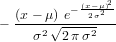
 - (x-μ)2- - (x--μ)√-e--2σ2-- σ2 2 πσ2
(3)

A Python function that gives a properly re-ordered first derivative is

def periodic_gaussian_deriv(x, sigma): 
    nx = len(x) 
    # put the peak in the middle of the array: 
    mu = x[nx/2] 
    g = dgaussiandx(x, mu, sigma) 
    # need to normalize, the discrete approximation will be a bit off: 
    g = g / (-sp.sum(x * g)) 
    # reorder to split the peak across the boundaries: 
    return(sp.append(g[nx/2:nx], g[0:nx/2]))

In the same way that we used the Gaussian for smoothing we can use its derivative for differentiation. Here’s the Python to do that:

# calculate some derivatives: 
sigma_deriv = 0.5 # this can be small because weve already smoothed a lot 
cyl_deriv = [] 
for i,c in enumerate(cyl_deconv_smooth): 
    cyl_deriv.append( 
        ifft(fft(c) * fft(periodic_gaussian_deriv(x, sigma_deriv*dx))).real)

Figure 5 shows the results. The wiggles that we don’t manage to smooth in the initial sharpening stage become amplified by differentiation.


PIC

Figure 5: Derivative of De-convolved Functions


Once we have a numerical approximation for the derivative, calculating the integral is straight-forward:

def abel(dfdx, x): 
    nx = len(x) 
    # do each half of the signal separately (they should be the same 
    # up to noise) 
    integral = sp.zeros((2,nx/2), dtype=float) 
    for i in xrange(nx/2, nx-1): 
        divisor = sp.sqrt(x[i:nx]**- x[i]**2) 
        integrand = dfdx[i:nx] / divisor 
        integrand[0] = integrand[1] # deal with the singularity at x=r 
        integral[0][i-nx/2] = - sp.trapz(integrand, x[i:nx]) / sp.pi 
    for i in xrange(nx/2, 1, -1): 
        divisor = sp.sqrt(x[i:0:-1]**- x[i]**2) 
        integrand = dfdx[i:0:-1] / divisor 
        integrand[0] = integrand[1] # deal with the singularity at x=r 
        integral[1][-i+nx/2] = - sp.trapz(integrand, x[i:0:-1]) / sp.pi 
    return(integral)

The one minor ’gotcha’ is dealing with the integrable singularity in 2. We just copy the value of the nearest neighbor over the Inf, the integral will approach the correct value in the limit of small Δx (lots of points).


PIC

Figure 6: Inverse Abel Transform Results


The analytical inverse Abel transform of the theoretical phase shift curve can be easily calculated (Maxima [4] script shown in section A.2). The theoretical phase shift has the form

 2 2 P (x) = width - (x- x0)
(4)

which gives the derivative as

∂P ∂x-= - 2 (x- x0)
(5)

and finally, the inverse Abel transform as

 2 (log(2 (√a2---r2 + a)) x0 - log (2 r) x0 - √a2---r2) p(r) = - ---------------------------------------------- π
(6)

2.1 Centering

Often, despite our best efforts, the data are not centered. There is a method to estimate the optimal shift required to center the data using the FFT [5]. Figure 7 shows one of the “measurements” shifted by a small amount.


PIC

Figure 7: Shifted Measurement


The method of Jaffe et al. [5] is to maximize

N∕2-1 ∑ [ -2πmk Δfn ]2 Re(e Lnh) -N ∕2
(7)

Where Lnh is the Fourier transform of the data, and mkΔ is a shift. Since the data is real, the real part of its transform is the even part of the signal. The shift which maximizes the magnitude of the even part is the one which makes the data most even (centered). A graphical analysis of the data can provide a range of shifts to try. The Python to perform this maximization is shown below (this relies on being able to index arrays with arrays of integers, which can be done in Matlab as well).

# a shifted measurement 
shift = nx / 10 # a ten percent shift 
cyl_shifted = cyl_conv[2][scipy.append(range(shift,nx), range(0,shift))] 
# find the shift needed to center the measurement (should match shift above): 
indices = [] 
# get range of shifts to try from eye-balling the measurement 
try_shift = range(nx - 2*shift, nx) 
for i in try_shift: 
    indices.append(scipy.append(range(i,nx), range(0,i)).astype(int)) 
even_norm = sp.zeros(len(indices), dtype=float) 
for i, cyclic_perm in enumerate(indices): 
    even_norm[i] = sp.sum(fft(cyl_shifted[cyclic_perm]).real**2) 
max_even_shift = try_shift[even_norm.argmax()]

Figure 8 shows that the objective function (equation 7) reaches a local maximum at the shift which was originally applied (shown in Figure 7).


PIC

Figure 8: Centering Objective Function


3 Calibration Model Fitting

The techniques presented in section 1 can be combined to fit a calibration model to interferometry measurements of a calibration cylinder (or any other object for which you have the theoretical phase-shift curve). The purpose of a calibration model is to provide estimates of parameters like the standard deviation of the Gaussian beam for use in deconvolution and inversion of subsequent test measurements.

There steps in fitting the model are

  1. Center the data (2.1)
  2. Find an error minimizing set of deconvolution and smoothing σs (these are the parameters of our model).
    1. Define a function of the data and the σs which returns an error norm between the theoretical phase shift curve and the smoothed, deconvolved data.
    2. Apply a minimization algorithm to this function. Choose an initial guess for the deconvolution σ which is likely to be smaller than the true σ.

The Python functions to accomplish this are shown below. One error function uses a sum of squared errors and the other uses a maximum error.

def smooth_deconv(s, x, data): 
    fsmooth = fft(data) * fft(periodic_gaussian(x, s[0])) 
    fdeconv = ifft(fsmooth / fft(periodic_gaussian(x, s[1]))).real 
    return(fdeconv) 
 
def cal_model_ls_err(s, x, data, theoretical): 
    fdeconv = smooth_deconv(s, x, data) 
    return(sp.sqrt(sp.sum((fdeconv - theoretical)**2))) 
 
def cal_model_minmax_err(s, x, data, theoretical): 
    fdeconv = smooth_deconv(s, x, data) 
    return((abs(fdeconv - theoretical)).max())

The error in the fitted model following this approach is shown in Figure 9. Both the least squares error and the min-max error methods recover the correct deconvolution σ.


PIC

Figure 9: Error in Calibration Fit


4 Further Improvements / Variations

Jaffe et al. [5] also suggest “symmetrizing” before calculating the Abel transform by removing the imaginary component of the transformed data. They also estimate the variance of the inverse Abel transform based on both the portion of the data removed by filtering (smoothing) and symmetrizing.

Rather than calculating the derivative necessary for the inverse Abel transform with a convolution, a pseudo-spectral method could be used. The trade-off being that very accurate derivatives could be attained at the expense of greatly amplifying any noise. A more practical variation, that is not susceptible to noise, would be to calculate the integral with a pseudo-spectral approach rather than the composite trapezoidal rule. This would give a more accurate integral, and bring the numerical and analytical curves in Figure 6 into closer agreement.

A Complete Scripts

A.1 Python

The complete Python script to do all of the calculations and generate all of the plots in this tutorial is available.

A.2 Maxima

The Maxima batch file used to calculate the inverse Abel transform of the theoretical phase-shift curve is available.

References

[1]   Hamming, R.W., “Numerical Methods for Scientists and Engineers,” 2nd. ed., Dover Publications, 1986.

[2]   Jones, E., Oliphant, T., Peterson, P., “Scipy: Open source scientific tools for Python,” 2001–, http://www.scipy.org

[3]   Hutchinson, I.H., “Principles of Plasma Diagnostics,” 2nd ed., Cambridge University Press, 2002.

[4]   Schelter, W., et al., “Maxima: a computer algebra system,” http://maxima.sourceforge.net

[5]   Jaffe, S.M., Larjo, J., Henberg, R., “Abel Inversion Using the Fast Fourier Transform,” 10th International Symposium on Plasma Chemistry, Bochum, (1991).