Showing posts with label Jaynes. Show all posts

Wednesday, October 23, 2013

Starcraft, Jaynes, and Bayesian UQ


Interesting content covered on Nuite Blanche of a recent Paris Machine Learning meetup. The work on applying Bayesian Programming and Learning for Multi-Player Video Games was really neat. It's about developing a bot for playing Starcraft. Some additional related presentations:
This problem is real enough to be interesting, and simple enough to tackle. I really liked how this work dealt with the separation of strategic/tactical level decision making.

Sunday, December 13, 2009

Jaynes on Outliers and Robustness

A few of the sections from Chapter 21 of Jayne’s book are reproduced below. The topic is such an important one to the practicing engineer / scientist, yet orthodox robust regression is a nearly impenetrable mess of ad hoceries. In comparison, the treatment of outliers is quite straight-forward in a Bayesian framework.

21.3 The two-model model

We have a ’good’ sampling distribution


G (x|θ)
(21.2)

with a parameter θ that we want to estimate. Data drawn urn-wise from G(x|θ) are called ’good’ data. But there is a ’bad’ sampling distribution


B (x|η)
(21.3)

possibly containing an uninteresting parameter η. Data from B(x|η) are called ’bad’ data; they appear to be useless or worse for estimating θ, since their probability of occurring has nothing to do with θ. Our data set consists of n observations


D = (x1,...,xn )
(21.4)

But the trouble is that some of these data are good and some are bad, and we do not know which (however, we may be able to make guesses: an obvious outlier – far out in the tails of G(x|θ) – or any datum in a region of x where G(x|θ) B(x|η) comes under suspicion of being bad).

In various real problems we may, however, have some prior information about the process that determines whether a given datum will be good or bad. Various probability assignments for the good/bad selection process may express that information. For example, we may define


 { 1 if the ith datum is good qi = 0 if the ith datum is bad
(21.5)

and then assign joint prior probabilities


p(q1⋅⋅⋅qn|I)<br />
(21.6)

to the 2n conceivable sequences of good and bad.


21.4 Exchangeable selection

Consider the most common case, where our information about the good/bad selection process can be represented by assigning an exchangeable prior. That is, the probability of any sequence of n good/bad observations depends only on the numbers r, (n - r) of good and bad ones, respectively, and not on the particular trials at which they occur. Then the distribution 21.6 is invariant under permutations of the qi, and by the de Finetti representation theorem (Chapter 18), it is determined by a single generating function
g(u):


 ∫ 1 r n- r p(q1⋅⋅⋅qn|I) = du u (1 - u ) g(u) 0
(21.7)

It is much like flipping a coin with unknown bias where, instead of ’good’ and ’bad’, we say ’heads’ and ’tails’. There is a parameter u such that if u were known we would say that any given datum x may, with probability u, have come from the good distribution; or with probability (1 - u) from the bad one. Thus, u measures the ’purity’ of our data; the closer to unity the better. But u is unknown, and g(u) may, for present purposes, be thought of as its prior probability density (as was, indeed, done already by Laplace; further technical details about this representation are given in Chapter 18). Thus, our sampling distribution may be written as a probability mixture of the good and bad distributions:


p(x |θ,η,u ) = uG (x|θ ) + (1 - u)B (x|η), 0 ≤ u ≤ 1
(21.8)

This is just a particular form of the general parameter estimation model, in which θ is the parameter of interest, while (η,u) are nuisance parameters; it requires no new principles beyond those expounded in Chapter 6.

Indeed, the model 21.8 contains the usual binary hypothesis testing problem as a special case, where it is known initially that all the observations are coming from G, or they are all coming from
B, but we do not know which. That is, the prior density for u is concentrated on the points u = 0,
u = 1:


p(u|I) = p0δ(1 - u) + p1δ (u )
(21.9)

where p0 = p(H0|I), p1 = 1 - p0 = p(H1|I) are the prior probabilities for the two hypotheses:


H0 ≡ all the data come from the distribution G(x |θ) H1 ≡ all the data come from the distribution B(x |η)
(21.10)

Because of their internal parameters, they are composite hypotheses; the Bayesian analysis of this case was noted briefly in Chapter 4. Of course, the logic of what we are doing here does not depend on value judgements like ’good’ or ’bad’.

Now consider u unknown and the problem to be that of estimating θ. A full non-trivial Bayesian solution tends to become intricate, since Bayes’ theorem relentlessly seeks out and exposes every factor that has the slightest relevance to the question being asked. But often much of that detail contributes little to the final conclusions sought (which might be only the first few moments, or percentiles, of a posterior distribution). Then we are in a position to seek useful approximate algorithms that are ’good enough’ without losing essential information or wasting computation on non-essentials. Such rules might conceivably be ones that intuition had already suggested, but, because they are good mathematical approximations to the full optimal solution, they may also be far superior to any of the intuitive devices that were invented without taking any note of probability theory; it depends on how good that intuition was.

Our problem of outliers is a good example of these remarks. If the good sampling density
G(x|θ) is very small for |x| < 1, while the bad one B(x|η) has long tails extending to |x|≫ 1, then any datum y for which |y| > 1 comes under suspicion of coming from the bad distribution, and intuitively one feels that we ought to ’hedge our bets’ a little by giving it, in some sense, a little less credence in our estimate of θ. Put more specifically, if the validity of a datum is suspect, then intuition suggests that our conclusions ought to be less sensitive to its exact value. But then wee have just about stated the condition of robustness (only now, this reasoning gives it a rationale that was previously missing). As |x|→∞ it is practically certain to be bad, and intuition probably tells us that we ought to disregard it altogether.

Such intuitive judgments were long since noted by Tukey and others, leading to such devices as the ’re-descending psi function’, which achieve robust/resistant performance by modifying the data analysis algorithms in this way. These works typically either do not deign to note even the existence of Bayesian methods, or contain harsh criticism of Bayesian methods, expressing a belief that they are not robust / resistant and that the intuitive algorithms are correcting this defect – but never offering any factual evidence in support of this position.

In the following we break decades of precedent actually examining a Bayesian calculation of outlier effects, so that one can see – perhaps for the first time – what Bayesianity has to say about the issue, and thus give that missing factual evidence.


21.5 The general Bayesian solution

Firstly, we give the Bayesian solution based on the model 21.8 in full generality, then we study some special cases. Let f(θηu|I) be the joint prior density for the parameters. Their joint posterior density given the data D is


f(θ, η, u|D I) = Af (θ, η, u|I) L (θ, η, u)
(21.11)

where A is a normalizing constant, and, from 21.8,


 n ∏ L (θ, η, u) = [uG (xi|θ) + (1 - u)B (xi|η )] i=1
(21.12)

is their joint likelihood. The marginal posterior density for θ is


 ∫ ∫<br />p(θ|D I) = d ηdu f(θ, η, u|D I)
(21.13)

To write 21.12 more explicitly, factor the prior density:


f (θ, η, u|I) = h(η, u|θ, I)f(θ|I)
(21.14)

where f(θ|I) is the prior density for θ, and h(η, u|θ, I) is the joint prior for (η,u), given θ. Then the marginal posterior density for θ, which contains all the information that the data and the prior information have to give us about θ, is
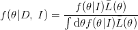


 f(θ|I)¯L(θ) f(θ|D, I) = ∫---------¯---- d θf(θ|I)L(θ)
(21.15)

where we have introduced the quasi-likelihood


 ∫∫<br />¯L (θ) = dηdu L (θ, η, u )h (η, u |θ, I)
(21.16)

Inserting 21.12 into 21.16 and expanding, we have


 [ ¯L(θ) = ∫∫ dηdu h (η, u |θ, I) unL(θ) + un- 1(1 - u) ∑n B (x |η)L (θ) n-2 2∑ j=1 j j +u (1 - u) j<k B (xj|η )B (xk|η)Ljk(θ) + ⋅⋅⋅ + (1 - u)nB (x1|η)⋅⋅⋅B (xn|η)]
(21.17)

in which


 ∏n L(θ) ≡ ∏ i=1 G(xi|θ) Lj(θ) ≡ ni⁄=j G(xi|θ) Lj(θ) ≡ ∏n G (xi|θ)... etc.  i⁄=j,k
(21.18)

are a sequence of likelihood functions for the good distribution in which we use all the data, all except the datum xj, all except xj and xk, and so on. To interpret the lengthy expression 21.17, note that the coefficient of L(θ),


∫ 1 ∫ ∫ du dη h(η, u|θ, I)un = du unh(u|θ, I) 0
(21.19)

is the probability, conditional on θ and the prior information, that all the data {x1,,xn} are good. This is represented in the Laplace-de Finetti form 21.7 in which the generating function g(u) is the prior density h(u|θ, I) for u, conditional on θ. Of course, in most real problems this would be independent of θ (which is presumably some parameter referring to an entirely different context than u); but preserving generality for the time being will help bring out some interesting points later.

Likewise, the coefficient of Lj(θ) in 21.17 is


∫ ∫ du un- 1(1 - u ) dη B(xj|η)h(η, u|θ, I)
(21.20)

now the factor


 ∫ n-1 d η du u (1 - u)h (η, u |θ I)
(21.21)

is the joint probability density, given I and θ, that any specified datum xj is bad, that the (n- 1) others are good, and that η lies in (η,η + dη). Therefore the coefficient 21.20 is the probability, given I and θ, that the jth datum would be bad and would have the value x
j
, and the other data would be good. Continuing in this way, we see that, to put it in words, our quasi-likelihood is:


¯L (θ ) = prob(all the data are good) × (likelihood using all the data) + ∑ prob(only xjbad) × (likelihood using all data except xj) ∑ j + j,k prob(only xj, xkbad ) × (likelihood using all except xj,xk) + ⋅∑⋅⋅ + j prob(only xj good) × (likelihood using only the datum xj) + prob(all the data are bad )
(21.22)

In shorter words: the quasi-likelihood L¯(θ) is a weighted average of the likelihoods for the good distribution G(x|θ) resulting from every possible assumption about which data are good, and which are bad, weighted according to the prior probabilities of those assumptions. We see how every detail of our prior knowledge about how the data are being generated is captured in the Bayesian solution.

This result has such wide scope that it would require a large volume to examine all its implications and useful special cases. But let us note how the simplest ones compare to our intuition.


21.6 Pure Outliers

Suppose the good distribution is concentrated in a finite interval


G (x|θ) = 0, |x| > 1
(21.23)

while the bad distribution is positive in a wider interval which includes this. Then any datum x for which |x| > 1 is known with certainty to be an outlier, i.e. to be bad. If |x| < 1, we cannot tell with certainty whether it is good or bad. In this situation our intuition tells us quite forcefully: Any datum that is known to be bad is just not part of the data relevant to estimation of θ and we shouldn’t be considering it at all. So just throw it out and base our estimate on the remaining data.

According to Bayes’ theorem this is almost right. Suppose we find xj = 1.432, xk = 2.176, and all the other x’s less than unity. Then, scanning 21.24 it is seen that only one term will survive:


 ∫ ∫ ¯ L(θ) = du dηh (η, u|θ, I)B (xj|η)B (xk |η)Ljk (θ ) = Cjk (θ)Ljk(θ)
(21.24)

As discussed above, the factor Cjk is almost always independant of θ, and since constant factors are irrelevant in a likelihood, our quasi-likelihood in 21.15 reduces to just the one obtained by throwing away the outliers, in agreement with that intuition.

But it is conceivable that in rare cases Cjk(θ) might, after all, depend on θ; and Bayes’ theorem tells us that such a circumstance would make a difference. Pondering this, we see that the result was to be expected if only we had thought more deeply. For if the probability of obtaining two outliers with values xj, xk depends on θ, then the fact that we got those particular outliers is in itself evidence relevant to inference about
θ.

Thus, even in this trivial case Bayes’ theorem tells us something that unaided intuition did not see: even when some data are known to be outliers, their values might still, in principle, be relevant to estimation of θ. This is an example of what we meant in saying that Bayes’ theorem relentlessly seeks out and exposes every factor that has any relevance at all to the question being asked.

In the more usual situations, Bayes’ theorem tells us that whenever any datum is known to be an outlier, then we should simply throw it out, if the probability of getting that particular outlier is independent of θ. For, quite generally, a datum xi can be known with certainty to be an outlier ony if G(xi|θ) = 0 for all θ; but in that case every likelihood in 21.24 that contains xi will be zero, and our posterior distribution for θ will be the same as if the datum xi had never been observed.


21.7 One receding datum

Now suppose the parameter of interest is a location parameter, and we have a sample of ten observations. But one datum xj moves away from the cluster of the others, eventually receding out 100 standard deviations of the good distribution G. How will our estimate of θ follow it? The answer depends on which model we specify.

Consider the usual model in which the sampling distribution is taken to be simply G(x|θ) with no mention of any other ’bad’ distribution. If G is Gaussian, x N(θ,σ), and our prior for θ is wide (say > 1000σ), then the Bayesian estimate for quadratic loss function will remain equal to the samaple average, and our far-out datum will pull the estimate about ten standard deviations away from the average indicated by the other nine data values. This is presumably the reason why Bayesian methods are sometimes charged with failure to be robust/resistant.

However, that is the result only for the assumed model, which in effect proclaims dogmatically: I know in advance that u = 1; all the data will come from G, and I am so certain of this that no evidence from the data could change my mind. If one actually had this much prior knowledge, then that far-out datum would be highly significant; to reject it as an ’outlier’ would be to ignore cogent evidence, perhaps the most cogent piece of evidence that the data provide. Indeed, it is a platitude that important scientific discoveries have resulted from an experiment having that much confidence in his apparatus, so that surprising new data were believed; and not merely rejected as ’accidental’ outliers.

If, nevertheless, our intuition tells us with overwhelming force that the deviant datum should be thrown out, then it must be that we do not really believe that u = 1 strongly enough to adhere to it in the face of the evidence of the surprising datum. A Bayesian may correct this by use of the more realistic model 21.8. Then the proper criticism of the first procedure is not of Bayesian methods, but rather of the saddling of Bayesian methodology with an inflexible, dogmatic model which denies the possibility of outliers. We saw in Section 4.4 on multiple hypothesis testing just how much difference it can make when we permit the robot to become skeptical about an overly simple model.

Bayesian methods have inherent in them all the desirable robust/resistant qualities, and they will exhibit these qualities automatically, whenever they are desirable – if a sufficiently flexible model permits them to do so. But neither Bayesian nor any other methods can give sensible results if we put absurd restrictions on them. There is a moral in this, extending to all of probability theory. In other areas of applied mathematics, failure to notice some feature (like the possibility of the bad distribution B) means only that it will not be taken into account. In probability theory, failure to notice some feature may be tantamount to making irrational assumptions about it.

Then why is it that Bayesian methods have been criticized more than orthodox ones on this issue? For the same reason that city B may appear in the statistics to have a higher crime rate than city A, when the fact is that city B has a lower crime rate, but more efficient means for detecting crime. Errors undetected are errors uncriticized.

Like any other problem in this field, this can be further generalized and extended endlessly, to a three-model model, putting parameters in 21.6, etc. But our model is already general enough to include both the problem of outliers and conventional hypothesis testing theory; and a great deal can be learned from a few of its simple special cases.

Friday, December 11, 2009

Dueling Bayesians

Percontations: The Nature of Probability

Interest points:

  • Fun with coin-flipping (13:43)

  • Can probabilistic thinking be completely automated? (04:31)

  • The limits of probability theory (11:07)

  • How Andrew got shot down by Daily Kos (06:55)

  • Is the academic world addicted to easy answers? (11:11)

    This part of the discussion was very brief, but probably the most interesting. What Gelman is referring to is maximum entropy sampling, or optimal sequential design of experiments. This has some cool implications for model validation I think (see below).

  • The difference between Eliezer and Nassim Taleb (06:20)


Links mentioned:


Some things Dr Gelman said that I think are interesting:

I was in some ways thinking like a classical statistician, which was, well,I'll be wrong 5% of the time, you know, that's life. We can be wrong a lot, but you're never supposed to knowingly be wrong in Bayesian statistics. If you make a mistake, you shouldn't know that you made a mistake, that's a complete no-no.


With great power comes great responsibility. [...] A Bayesian inference can create predictions of everything, and as a result you can be much more wrong as a Bayesian than as a classical statistician.


When you have 30 cases your analysis is usually more about ruling things out than proving things.

Towards the end of the discussion Yudowski really sounds like he's parroting Jaynes (maybe they are just right in the same way).

Bayesian design of validation experiments

As I mentioned in the comments about the Gelman/Yudowski discussion, the most interesting thing to me was the ’adaptive testing’ that Gelman mentioned. This is a form of sequential design of experiments , and the Bayesian versions are the most flexible. That is because Bayes theorem provides a consistent and coherent (if not always conveneint) way of updating our knowledge state as each new test result arrives. Then, and Gelman’s comment about ’making predictions about everything’ is germane here, we assess our predictive distributions and find the areas of our parameter space that have the most uncertainty (highest entropy of the predictive distribution). This place in our parameter space with the highest predictive distribution entropy is where we should test next to get the most information. The example of academic testing that Gelman gives does exactly that, the question chosen is the one that the test-taker has equal chance of getting right or wrong.

The same idea applies to testing to validate models. Here’s a little passage from a relevant paper that provides some background and motivation [1]:

Under the constraints of time, money, and other resources, validation experiments often need to be optimally designed for a clearly defined purpose, namely computational model assessment. This is inherently a decision theoretic problem where a utility function needs to be first defined so that the data collected from the experiment provides the greatest opportunity for performing conclusive comparisons in model validation.

The method suggested to achieve this is based on choosing a test point from the area of the parameter space with the highest predictive entropy and also one from the area with the lowest predicitive entropy [2]. This addresses the little comment Gelman made about not being able to asses the goodness of the model very well if you only choose points in the high entropy area. Each round of two test points gives you an opportunity to make the most conclusive comparison of the model prediction to reality.

If you were just trying to calibrate a model, then you would only want to choose test points in the high-entropy-areas because these would do the most to reduce your uncertainty about the reality of interest (and hence give you better parameter estimates). Since we are trying to validate the model though, we want to evaluate its performance where we expect it to give the best predictions and where we expect it to give the worst predictions. Here the idea explained in a bit more technical language [1]:

Consider the likelihood ratio Λ(y) in Eq. (9) [or Bayes factor in [6]] as a validation metric. Suppose an experiment is conducted with the minimization result, and the experimental output is compared with model prediction. We expect a high value Λ(y)min , where the subscript min indicates that the likelihood is obtained from the experimental output in the minimization case. If Λ(y)min < η, then clearly this experiment rejects the model, since the validation metric Λ(y), even under the most favorable conditions, does not meet the threshold value η. On the other hand, suppose an experiment is conducted with the maximization result, and the experimental output is compared with the model prediction. We expect a low value Λ(y)max < η in this case. If Λ(y)max > η, then clearly this experiment accepts the model, since it is performed under the worst condition and still produces the validation metric to be higher than η. Thus, the cross entropy method provides conclusive comparison as opposed to an experiment at any arbitrary point.


Here's a graphical depiction of the placement of the optimal Bayesian decision boundary (image taken from [3]):


It would be nice to see these sorts of decision theory concepts applied to the public policy decisions that are being driven by the output of computational physics codes.

References

[1] Jiang, X., Mahadevan, S., “Bayesian risk-based decision method for model validation under uncertainty,” Reliability Engineering & System Safety, No. 92, pp 707-718, 2007.

[2] Jiang, X., Mahadevan, S., “Bayesian cross entropy methodology for optimal design of validation experiments,” Measurement Science & Technology, 2006.

[3] Jiang, X., Mahadevan, S., “Bayesian validation assessment of multivariate computational models ,” Journal of Applied Statistics, Vol. 35, No. 1, Jan 2008.

Monday, December 7, 2009

Final Causes

This is the conclusion of the comments section in the model comparison chapter (Chapter 20) from Jayne’s book (emphasis original).


It seems that every discussion of scientific inference must deal, sooner or later, with the issue of belief or disbelief in final causes. Expressed views range all the way from Jaques Monod (1970) forbidding us even to mention purpose in the Universe, to the religious fundamentalist who insists that it is evil not to believe in such a purpose. We are astonished by the dogmatic, emotional intensity with which opposite views are proclaimed, by persons who do not have a shred of supporting factual evidence for their positions.

But almost everyone who has discussed this has supposed that by a ’final cause’ one means some supernatural force that suspends natural law and takes over control of events (that is, alters positions and velocities of molecules in a way inconsistent with the equations of motions) in order to ensure that some desired final condition is attained. In our view, almost all past discussions have been flawed by failure to recognize that operation of a final cause does not imply controlling molecular details.

When the author of a textbook says: ’My purpose in writing this book was to…’, he is disclosing that there was a true ’final cause’ governing many activities of writer, pen, secretary, word processor, extending usually over several years. When a chemist imposes conditions on his system which forces it to have a certain volume and temperature, he is just as truly the wielder of a final cause dictating the final thermodynamic state that he wished it to have. A bricklayer and a cook are likewise engaged in the art of invoking final causes for definite purposes. But – and this is the point almost always missed – these final causes are macroscopic; they do not determine any particular ’molecular’ details. In all cases, had those fine details been different in any one of billions of ways, the final cause would have been satisfied just as well.

The final cause may then be said to possess an entropy, indicating the number of microscopic ways in which its purpose can be realized; and the larger that entropy, the greater is the probability that it will be realized. Thus the principle of maximum entropy applies also here.

In other words, while the idea of a microscopic final cause runs counter to all the instincts of a scientists, a macroscopic final cause is a perfectly familiar and real phenomenon, which we all invoke daily. We can hardly deny the existence of purpose in the Universe when virtually everything we do is done with some definite purpose in mind. Indeed, anybody who fails to pursue some definite long-term purpose in the conduct of his life is dismissed as an idler by his colleagues. Obviously, this is just a familiar fact with no religious connotations – and no anti-religious ones. Every scientist believes in macroscopic final causes without thereby believing in supernatural contravention of the laws of physics. The wielder of the final cause is not suspending physical law; he is merely choosing the Hamiltonian with which some system evolves according to physical law. To fail to see this is to generate the most fantastic, mystical nonsense.


So we have the wager from Pascal, and God as the ultimate ’Hamiltonian chooser’ from Jaynes?

Sunday, December 6, 2009

Sociology of Science

This is the first part of the comments section in the model comparison chapter (Chapter 20) from Jayne’s book (emphasis mine).

Actual scientific practice does not really obey Ockham’s razor, either in its previous ’simplicity’ form or in our revised ’plausibility’ form. As so many of us have deplored, the attractive new hypothesis or model, which accounts for the facts in such a neat, plausible way that you want to believe it at once, is usually pooh-poohed by the official Establishment in favor of some drab, complicated, uninteresting one; or, if necessary, in favor of no alternative at all. The progress of science is carried forward mostly by the few fundamental dissenting innovators, such as Copernicus, Galileo, Newton, Laplace, Darwin, Mendel, Pasteur, Boltzmann, Einstein, Wegener, Jeffreys – all of whom had to undergo this initial rejection and attack. In the cases of Galileo, Laplace, and Darwin, these attacks continued for more than a century after their deaths. This is not because their new hypothesis were faulty – quite the contrary – but because this is the part of the sociology of science (and, indeed of all scholarship). In any field, the Establishment is seldom in pursuit of the truth, because it is composed of those who sincerely believe that they are already in possession of it.

The sociology of science is an interesting topic that’s been brought forcefully into the public perception by the recent kerfuffle over the leaked UEA CRU emails. Hans von Storch has an interesting guest post over on Roger Pielke’s site discussing some of the concerns along with suggestions for improving the sustainability of science.

I think ’sustainability of science’ is his way of saying maintaining long-term credibility. Being honest about the uncertainties and not using science to support a ’preconceived political agenda of something good’. This is an unarguably good thing. A hard thing for sure, but something no one would argue against out loud. The term Pielke gives for the behaviour exhibited by the CRU scientists is ’stealth advocacy’. When you wrap the mantle of Science (relevant Anchorman audio clip, it really is relevant, the relevant part is at the very end) around your advocacy and misrepresent the actual state of knowledge to decision makers and laypeople, then you aren’t living up to that particular sort of honesty that Feynman exhorted scientists to uphold.

Wednesday, November 25, 2009

Converging and Diverging Views

I was brushing up on my maximum entropy and probability theory the other day and came across a great passage in Jaynes' book about convergence and divergence of views. He applies basic Bayesian probability theory to the concept of changing public opinion in the face of new data, especially the effect prior states of knowledge (prior probabilities) can have on the dynamics. The initial portion of section 5.3 is reproduced below.

5.3 Converging and diverging views (pp. 126 – 129)

Suppose that two people, Mr A and Mr B have differing views (due to their differing prior information) about some issue, say the truth or falsity of some controversial proposition S. Now we give them both a number of new pieces of information or ’data’, D1,D2,,Dn, some favorable to S, some unfavorable. As n increases, the totality of their information comes to be more nearly the same, therefore we might expect that their opinions about S will converge toward a common agreement. Indeed, some authors consider this so obvious that they see no need to demonstrate it explicitly, while Howson and Urbach (1989, p. 290) claim to have demonstrated it.

Nevertheless, let us see for ourselves whether probability theory can reproduce such phenomena. Denote the prior information by IA, IB, respectively, and let Mr A be initially a believer, Mr B be a doubter:


P (S|IA) ≃ 1, P(S |IB ) ≃ 0
(5.16)

after receiving data D, their posterior probabilities are changed to


 P (D |SIA) P(S |D IA) = P (S|IA)---------- P (D |IA )
(5.17)


 P-(D-|SIB-) P(S |D IB) = P (S|IB) P (D |IB )
(5.17)

If D supports S, then since Mr A already considers S almost certainly true, we have P(D|S IA), and so


P (S |D IA) ≃ P (S |IA)
(5.18)

Data D have no appreciable effect on Mr A’s opinion. But now one would think that if Mr B reasons soundly, he must recognize that P(D|S IB) > P(D|IB), and thus


P (S |D I ) > P (S |I ) B B
(5.19)

Mr B’s opinion should be changed in the direction of Mr A’s. Likewise, if D had tended to refute
S, one would expect that Mr B’s opinions are little changed by it, whereas Mr A’s will move in the direction of Mr B’s. From this we might conjecture that, whatever the new information D, it should tend to bring different people into closer agreement with each other, in the sense that


|P (S|D I ) - P (S |D I )| < |P (S|I ) - P (S|I )| A B A B
(5.20)

Although this can be verified in special cases, it is not true in general.

Is there some other measure of ‘closeness of agreement’ such as log[P(S|D Ia)∕P(S|D IB], for which this converging of opinions can be proved as a general theorem? Not even this is possible; the failure of probability theory to give this expected result tells us that convergence of views is not a general phenomenon. For robots and humans who reason according to the consistency desiderata of Chapter 1, something more subtle and sophisticated is at work.

Indeed, in practice we find that this convergence of opinions usually happens for small children; for adults it happens sometimes but not always. For example, new experimental evidence does cause scientists to come into closer agreement with each other about the explanation of a phenomenon.

Then it might be thought (and for some it is an article of faith in democracy) that open discussion of public issues would tend to bring about a general consensus on them. On the contrary, we observe repeatedly that when some controversial issue has been discussed vigorously for a few years, society becomes polarized into opposite extreme camps; it is almost impossible to find anyone who retains a moderate view. The Dreyfus affair in France which tore the nation apart for 20 years, is one of the most thoroughly documented examples of this (Bredin, 1986). Today, such issues as nuclear power, abortion, criminal justice, etc., are following the same course. New information given simultaneously to different people may cause a convergence of views; but it may equally well cause a divergence.

This divergence phenomenon is observed also in relatively well-controlled psychological experiments. Some have concluded that people reason in a basically irrational way; prejudices seem to be strengthened by new information which ought to have the opposite effect. Kahneman and Tversky (1972) draw the opposite conclusion from such psychological tests, and consider them an argument against Bayesian methods.

But now in view of the above ESP example, we wonder whether probability theory might also account for this divergence and indicate that people may be, after all, thinking in a reasonably rational, Bayesian way (i.e. in a way consistent with their prior information and prior beliefs). The key to the ESP example is that our new information was not

S fully adequate precautions against error or deception were taken, and Mrs Stewart did in fact deliver that phenomenal performance.

It was that some ESP researcher has claimed that S is true. But if our prior probability for S is lower than our prior probability that we are being deceived, hearing this claim has the opposite effect on our state of belief from what the claimant intended.

The same is true in science and politics; the new information a scientist gets is not that an experiment did in fact yield this result, with adequate protection against error. It is that some colleague has claimed that it did. The information we get from TV evening news is not that a certain event actually happened in a certain way; it is that some news reporter claimed that it did.

Scientists can reach agreement quickly because we trust our experimental colleagues to have high standards of intellectual honesty and sharp perception to detect possible sources of error. And this belief is justified because, after all, hundreds of new experiments are reported every month, but only about once in a decade is an experiment reported that turns out later to have been wrong. So our prior probability for deception is very low; like trusting children, we believe what experimentalists tell us.

In politics, we have a very different situation. Not only do we doubt a politician’s promises, few people believe that news reporters deal truthfully and objectively with economic, social, or political topics. We are convinced that virtually all news reporting is selective and distorted, designed not to report the facts, but to indoctrinate us in the reporter’s socio-political views. And this belief is justified abundantly by the internal evidence in the reporter’s own product – every choice of words and inflection of voice shifting the bias invariably in the same direction.

Not only in political speeches and news reporting, but wherever we seek for information on political matters, we run up against this same obstacle; we cannot trust anyone to tell us the truth, because we perceive that everyone who wants to talk about it is motivated either by self-interest or by ideology. In political matters, whatever the source of information, our prior probability for deception is always very high. However, it is not obvious whether this alone can prevent us from coming to agreement.

Jaynes, E.T., Probability Theory: The Logic of Science (Vol 1), Cambridge University Press, 2003.