Wow, the user friendliness and speed of this app is just amazing. A long way in ease and useability from the open source tool chain I've used previously.
Showing posts with label image processing. Show all posts
Showing posts with label image processing. Show all posts
Wednesday, May 26, 2021
Tuesday, January 5, 2021
Machine Learning for Fluid Dynamics: Patterns
The data set he mentions is Johns Hopkins Turbulence Databases. Many hundreds of Terabytes of direct numerical simulations with different governing equations and boundary conditions.
Saturday, April 6, 2019
3D Shape Segmentation With Projective Convolutional Networks
This is an interesting summary of an approach for shape segmentation. I think it's pretty cool how often VGG-16 gets used for transfer learning with good results. It's amazing that these models can represent enough knowledge to generate 3-D surfaces from single images. (I also like how many folks use airplanes as examples : - )
There's a website for the ShapeNet data set that they used as a benchmark in the video, and this paper describes the initial methods folks developed during the challenge right after the data set was released. That's a pretty neat approach. It reminds me a bit of the AIAA drag prediction workshops.
There's a website for the ShapeNet data set that they used as a benchmark in the video, and this paper describes the initial methods folks developed during the challenge right after the data set was released. That's a pretty neat approach. It reminds me a bit of the AIAA drag prediction workshops.
Friday, November 10, 2017
Deep Learning to Accelerate Topology Optimization
 |
| Topology Optimization Data Set for CNN Training |
Saturday, October 19, 2013
Drone Swarm Photogrammetry of the Matterhorn
senseFly mapped the Matterhorn with a bunch of little UAVs. Pretty impressive photogrammetric point cloud: 300 million points!
Wednesday, March 6, 2013
GBU-8 Photogrammetry
More photogrammetry. This uses the same software tool chain I described before. Still needs a bit of work on surface reconstruction. I always underestimate how many pictures are needed to get a reasonable point cloud: more is better.
I took the pictures of the GBU-8 at the NMUSAF. The surprising thing to me was the landing gear on the aircraft in the background showing up so well.
I took the pictures of the GBU-8 at the NMUSAF. The surprising thing to me was the landing gear on the aircraft in the background showing up so well.
Sunday, February 17, 2013
Dayton Masonic Temple Photogrammetry
 |
| Bundler-PMVS2 Dense Point Cloud Visualization in Meshlab |
Monday, October 3, 2011
J2X Time Series
I thought the intermittent splashing of the cooling water/steam in the close-up portion of this J2-X engine test video looked interesting.
So, I used mplayer to dump frames from the video (30 fps) to jpg files (about 1800 images), and the Python Image Library to crop to a rectangle focused on the splashes.
 When a splash occurs the pixels in this region become much whiter, so the whiteness of the region should give an indication of the "splashiness". I then converted the images to black and white, and averaged the pixel values to get a scalar time-series. The whole time series is shown in the plot below.
 Also, here's a text file if you want to play with the data.
 Here's a PSD and autocorrelation for the section of the data excluding the start-up and shut-down transients.

 Here's a recurrence plot of that section of the data.
 This is a pretty short data set, but you can see that there are little "bursts" of periodic response in the recurrence plot (compare to some of the recurrence plots for Lorenz63 trajectories). I'm pretty sure this is not significant to engine development in any way, but I thought it was a neat source of time series data.
So, I used mplayer to dump frames from the video (30 fps) to jpg files (about 1800 images), and the Python Image Library to crop to a rectangle focused on the splashes.


Sunday, February 8, 2009
Unblurring Images
Tikhonov regularization is a pretty cool concept when applied to image processing. It lets you 'de-blur' an image, which is an ill-posed problem. The results won't be as spectacular as CSI, but still cool nonetheless.
 The original image, CSI fans pretend it is a license plate or a criminal's face in a low quality surveillance video, was made by taking a screenshot of some words in a word processor. The image doesn't have to be character based, but characters make good practice problems.
We then blur the image with a Toeplitz matrix. In Octave that's pretty easy:
im = imread("foo-fiddle.png");
[m, n] = size(im);
sigma_true = 10;
p = exp(-(0:n-1).^2 / (2 * sigma_true^2))';
p = p + [0; p(n:-1:2)];
p = p / sum(p);
G_true = toeplitz(p);
im = G_true*double(im)*G_true';

Generally after doing some floating point operations on an image you won't end up with something still scaled between 0 and 255, so the little function shown below rescales a vector's values to the proper range for a grayscale image.
function im = image_rescale(double_vector)
%% scale values linearly to lie between 0 and 255
m = max(double_vector);
n = min(double_vector);
scale = max(double_vector) - min(double_vector);
im = double_vector - (min(double_vector) + scale/2);
im = im ./ scale;
im = (255 .* im) + 127.5;
endfunction
This is where the regularization comes in. Since the problem is poorly conditioned we can't just recover the image by straightforward inversion. We'll use the singular value decomposition of our blurring matrix to create a regularized inverse, this is similar to the pseudoinverse. If the singular value decomposition of the blurring matrix is

Then the regularized inverse is

Where the entries in the diagonal matrix are given by

So as alpha approaches zero we approach the un-regularized problem. Chapter 4 of Watkins has good coverage of doing SVDs in Matlab. The Octave to perform this process is shown below in the function
function im_tik = tik_reg(im,sigma,alpha)
[m,n] = size(im);
p = exp(-(0:n-1).^2 / (2 * sigma^2))';
p = p + [0; p(n:-1:2)];
p = p / sum(p);
G = toeplitz(p);
[U, S, V] = svd(G,0);
Sinv = S / (S^2 + alpha*eye(length(S),length(S))^2);
im_tik = V*Sinv*U'*double(im)*V*Sinv*U';
endfunction
This gives us two parameters (sigma and alpha) we have to guess in a real image processing problem (because we won't be the ones blurring the original). Another weakness of the method is that we assumed we knew the model that produced the blur, if the real physical process that caused the blur is not similar to Gaussian noise, then we won't be able to extract the original image.
Here's a couple for-loops in Octave that try several combinations of alpha and sigma.
sigma = [9,10,11];
alpha = [1e-6,1e-7,1e-8];
for j = 1:length(sigma)
for i = 1:length(alpha)
unblur = tik_reg(im, sigma(j), alpha(i));
unblur = reshape(image_rescale(reshape(unblur,m*n,1)),m,n);
fname = sprintf("unblur_%d%d.png",i,j);
imwrite(fname, uint8(unblur));
endfor
endfor

Optical character recognition probably wouldn't work on the output, but a person can probably decipher what the original image said.
Original
 The original image, CSI fans pretend it is a license plate or a criminal's face in a low quality surveillance video, was made by taking a screenshot of some words in a word processor. The image doesn't have to be character based, but characters make good practice problems.
 Blurring
We then blur the image with a Toeplitz matrix. In Octave that's pretty easy:
im = imread("foo-fiddle.png");
[m, n] = size(im);
sigma_true = 10;
p = exp(-(0:n-1).^2 / (2 * sigma_true^2))';
p = p + [0; p(n:-1:2)];
p = p / sum(p);
G_true = toeplitz(p);
im = G_true*double(im)*G_true';

Generally after doing some floating point operations on an image you won't end up with something still scaled between 0 and 255, so the little function shown below rescales a vector's values to the proper range for a grayscale image.
function im = image_rescale(double_vector)
%% scale values linearly to lie between 0 and 255
m = max(double_vector);
n = min(double_vector);
scale = max(double_vector) - min(double_vector);
im = double_vector - (min(double_vector) + scale/2);
im = im ./ scale;
im = (255 .* im) + 127.5;
endfunction
De-Blurring
This is where the regularization comes in. Since the problem is poorly conditioned we can't just recover the image by straightforward inversion. We'll use the singular value decomposition of our blurring matrix to create a regularized inverse, this is similar to the pseudoinverse. If the singular value decomposition of the blurring matrix is

Then the regularized inverse is

Where the entries in the diagonal matrix are given by

So as alpha approaches zero we approach the un-regularized problem. Chapter 4 of Watkins has good coverage of doing SVDs in Matlab. The Octave to perform this process is shown below in the function
tik_reg().function im_tik = tik_reg(im,sigma,alpha)
[m,n] = size(im);
p = exp(-(0:n-1).^2 / (2 * sigma^2))';
p = p + [0; p(n:-1:2)];
p = p / sum(p);
G = toeplitz(p);
[U, S, V] = svd(G,0);
Sinv = S / (S^2 + alpha*eye(length(S),length(S))^2);
im_tik = V*Sinv*U'*double(im)*V*Sinv*U';
endfunction
This gives us two parameters (sigma and alpha) we have to guess in a real image processing problem (because we won't be the ones blurring the original). Another weakness of the method is that we assumed we knew the model that produced the blur, if the real physical process that caused the blur is not similar to Gaussian noise, then we won't be able to extract the original image.
Here's a couple for-loops in Octave that try several combinations of alpha and sigma.
sigma = [9,10,11];
alpha = [1e-6,1e-7,1e-8];
for j = 1:length(sigma)
for i = 1:length(alpha)
unblur = tik_reg(im, sigma(j), alpha(i));
unblur = reshape(image_rescale(reshape(unblur,m*n,1)),m,n);
fname = sprintf("unblur_%d%d.png",i,j);
imwrite(fname, uint8(unblur));
endfor
endfor

Optical character recognition probably wouldn't work on the output, but a person can probably decipher what the original image said.
Saturday, January 3, 2009
Thresholding for Edge Detection
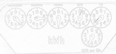
The real world is noisy, and the differencing operations of edge detection tend to magnify that noise. We can apply some statistical methods to our edge detection to hopefully overcome that. A very basic approach is to threshold based on a histogram of the gradient magnitude. Taking a look at the distribution of gradient magnitude for our trusty old electricity meter (shown below), it looks like a pixel level below about 235 puts us safely out into the tail of the distribution. Most pixels (in this image) are not edge pixels, so they are clustered on the high end of the scale.

This is pretty easy to do with
import numpy
import Image
pix = numpy.array( img.getdata() )
for i in xrange(0,pix.size):
if pix[i] < 235: pix[i] = 0 else: pix[i] = 255 img_out.putdata( pix )
Of course the histogram shape will depend on how much noise and how many edges are in the particular picture. This one had black dials on a white background, and not much noise so thresholding is a pretty fruitful strategy for really pulling out the edges.

You can make an intuitive argument that gradient magnitude distributions will have roughly similar shapes to that shown above. Especially as image resolutions steadily increase, the vast majority of pixels will not be on an edge. Sort of the curse of dimensionality in reverse, I guess that makes it a blessing.

This is pretty easy to do with
numpy and Image (PIL):import numpy
import Image
pix = numpy.array( img.getdata() )
for i in xrange(0,pix.size):
if pix[i] < 235: pix[i] = 0 else: pix[i] = 255 img_out.putdata( pix )
Of course the histogram shape will depend on how much noise and how many edges are in the particular picture. This one had black dials on a white background, and not much noise so thresholding is a pretty fruitful strategy for really pulling out the edges.

You can make an intuitive argument that gradient magnitude distributions will have roughly similar shapes to that shown above. Especially as image resolutions steadily increase, the vast majority of pixels will not be on an edge. Sort of the curse of dimensionality in reverse, I guess that makes it a blessing.
Wednesday, December 31, 2008
Treating Image Edges
There are some good examples floating around of creating customized image processing kernels in the python imaging library (PIL). It's very convenient to simply define your own mask, and the library takes care of the convolution.
One drawback is that the edges don't get filtered in this process. There are various ad-hoc things you can do. You can just drop a line of pixels all the way around the picture, so the gradient image of a 800x600 picture would be 798x598 pixels (if you're using a compact stencil), or you could just copy the edge pixels from the old picture to the new picture. So in effect, the edges don't get filtered. For most applications this is probably no big deal, but it might be, and we can do better.
All we have to do is change our difference operator for the edge pixels, use a forward or backward difference on the edges rather than the central differences used on the interior. Then you get gradient info for your edge pixels too!
Customizing the PIL kernel class has been done, so I'm going to use Fortran90 and F2Py for my difference operators. I'll still use the PIL for all of the convenient image reading/writing utilities though. No need to implement that in Fortran!
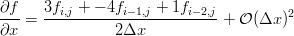
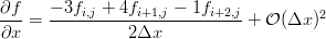
We can use our little Maxima script to generate the differences we need on the edges. If you've taken a basic numerical methods course you'll probably recognize them as the three point forward and backward difference approximations for the first derivative.
The Python to do just that is here:
import sys, math, Image, numpy
from filters import *
if __name__ == '__main__':
in_img = Image.open(sys.argv[1])
in_img = in_img.convert("L")
out_img = Image.new("L", in_img.size)
pix = in_img.getdata()
# put the pixels into a fortran contiguous array:
pix_array = numpy.array(pix)
pix_array = pix_array.reshape( in_img.size, order='F' )
# calculate the gradient
g = first_order_gradient(pix_array,in_img.size[0],in_img.size[1])
gmag = 255 - numpy.sqrt( g[0,:,:]*g[0,:,:] + g[1,:,:]*g[1,:,:] )
gmag.astype("int")
# pack the gradient magnitude into a new image
out_img.putdata( gmag.reshape( gmag.size, order='F' ) )
out_img.save(sys.argv[2])
Where I've used F2Py to generate the
! apply the central operator to the interior pixels
do j = 2, nj-1
do i = 2, ni-1
g(1,i,j) = (in_image(i+1,j) - in_image(i-1,j)) / 2.0
g(2,i,j) = (in_image(i,j+1) - in_image(i,j-1)) / 2.0
end do
end do
The gradients along the edges are calculated using the forward and backward differences (only x edges shown for brevity):
! loop over the y dimension and apply the asymmetric operators to the
! x min and x max edges
do j = 2, nj-1 ! leave out the corners
i = 1 ! minimum edge, go forward
g(1,i,j) = (-3.0*in_image(i,j) + 4.0*in_image(i+1,j) - in_image(i+2,j))/2.0
i = ni ! maximum edge, go backward
g(1,i,j) = (3.0*in_image(i,j) - 4.0*in_image(i-1,j) + in_image(i-2,j))/2.0
! no change for the y derivative
i = 1
g(2,i,j) = (in_image(i,j+1) - in_image(i,j-1)) / 2.0
i = ni
g(2,i,j) = (in_image(i,j+1) - in_image(i,j-1)) / 2.0
end do
Finally the four corners are calculated separately, because each one has a unique combination of stencils required. Putting the loops in Fortran speeds things up considerably compared to the pure Python implementations I did before. Here is the gradient magnitude of the dials from Poor Man's ADC calculated with the above technique:
One drawback is that the edges don't get filtered in this process. There are various ad-hoc things you can do. You can just drop a line of pixels all the way around the picture, so the gradient image of a 800x600 picture would be 798x598 pixels (if you're using a compact stencil), or you could just copy the edge pixels from the old picture to the new picture. So in effect, the edges don't get filtered. For most applications this is probably no big deal, but it might be, and we can do better.
All we have to do is change our difference operator for the edge pixels, use a forward or backward difference on the edges rather than the central differences used on the interior. Then you get gradient info for your edge pixels too!
Customizing the PIL kernel class has been done, so I'm going to use Fortran90 and F2Py for my difference operators. I'll still use the PIL for all of the convenient image reading/writing utilities though. No need to implement that in Fortran!
We can use our little Maxima script to generate the differences we need on the edges. If you've taken a basic numerical methods course you'll probably recognize them as the three point forward and backward difference approximations for the first derivative.


The Python to do just that is here:
import sys, math, Image, numpy
from filters import *
if __name__ == '__main__':
in_img = Image.open(sys.argv[1])
in_img = in_img.convert("L")
out_img = Image.new("L", in_img.size)
pix = in_img.getdata()
# put the pixels into a fortran contiguous array:
pix_array = numpy.array(pix)
pix_array = pix_array.reshape( in_img.size, order='F' )
# calculate the gradient
g = first_order_gradient(pix_array,in_img.size[0],in_img.size[1])
gmag = 255 - numpy.sqrt( g[0,:,:]*g[0,:,:] + g[1,:,:]*g[1,:,:] )
gmag.astype("int")
# pack the gradient magnitude into a new image
out_img.putdata( gmag.reshape( gmag.size, order='F' ) )
out_img.save(sys.argv[2])
Where I've used F2Py to generate the
filters module from a Fortran90 file. The module defines the subroutine first_order_gradient(), which implements the ideas discussed above. The gradients on the interior points are calculated using a central difference:! apply the central operator to the interior pixels
do j = 2, nj-1
do i = 2, ni-1
g(1,i,j) = (in_image(i+1,j) - in_image(i-1,j)) / 2.0
g(2,i,j) = (in_image(i,j+1) - in_image(i,j-1)) / 2.0
end do
end do
The gradients along the edges are calculated using the forward and backward differences (only x edges shown for brevity):
! loop over the y dimension and apply the asymmetric operators to the
! x min and x max edges
do j = 2, nj-1 ! leave out the corners
i = 1 ! minimum edge, go forward
g(1,i,j) = (-3.0*in_image(i,j) + 4.0*in_image(i+1,j) - in_image(i+2,j))/2.0
i = ni ! maximum edge, go backward
g(1,i,j) = (3.0*in_image(i,j) - 4.0*in_image(i-1,j) + in_image(i-2,j))/2.0
! no change for the y derivative
i = 1
g(2,i,j) = (in_image(i,j+1) - in_image(i,j-1)) / 2.0
i = ni
g(2,i,j) = (in_image(i,j+1) - in_image(i,j-1)) / 2.0
end do
Finally the four corners are calculated separately, because each one has a unique combination of stencils required. Putting the loops in Fortran speeds things up considerably compared to the pure Python implementations I did before. Here is the gradient magnitude of the dials from Poor Man's ADC calculated with the above technique:

Tuesday, December 30, 2008
Sobel, Scharr and Truncation Error
In image processing the discrete difference operators to calculate gradients and second derivatives are called "masks". They are often referred to as "stencils" in other applications of finite differences for solving PDEs, estimating sensitivities, etc.
Some of the kernels (a mask plus particular values) for calculating gradients are Sobel:
[ 1 2 1]
Gy = [ 0 0 0]
[-1 -2 -1]
[ 1 0 -1]
Gx = [ 2 0 -2]
[ 1 0 -1]
or Sharr:
[ 3 10 3]
Gy = [ 0 0 0]
[-3 -10 -3]
[ 3 0 -3]
Gx = [ 10 0 -10]
[ 3 0 -3]
or the simpler stencil we used in the previous posts, which only used neighbouring pixels in one direction to estimate the gradient. What if we want to design our own masks? A useful tool is the multidimensional Taylor series:

In two dimensions we have:

which includes up to third order terms. We can't actually include the two pure third order terms because we only have three points in either the x or y direction, and we need a minimum of four. We can include the mixed third order terms though, so that gives us 8 constraints on our coefficients. Instead of including all 9 points in the stencil we have to drop one, so in the Maxima code below you'll notice that the central point is commented out.
Lets examine the truncation error for the two masks above. First we define a vector of delta x and delta y corresponding to each point in the stencil:
/* define the points in the stencil or mask: */
steps : matrix( /* dx, dy */
[-1, 1],
[0, 1],
[1, 1],
[-1, 0],
/* [0,0], */
[1, 0],
[-1, -1],
[0,-1],
[1, -1] );
Then vectors describing the coefficients in the two masks (we'll just use the y-component for this example):
/* coefficients in sobel mask */
sobel_y : matrix(
[1],
[2],
[1],
[0],
/*[0],*/
[0],
[-1],
[-2],
[-1]
);
/* coefficients in sharr mask */
sharr_y : matrix(
[3],
[10],
[3],
[0],
/*[0],*/
[0],
[-3],
[-10],
[-3]
);
To evaluate the truncation error we also need to create an operator that is based on the multidimensional Taylor series shown above. This will let us simply multiply those vectors by the operator to see what the masks are actually estimating. Here's the operator:
n : matrix_size( steps );
A : zeromatrix(n[1],n[1]);
for j : 1 thru n[1] do ( A[1,j] : 1 );/* f */
for j : 1 thru n[1] do ( A[2,j] : steps[j,1] );/* df/dx */
for j : 1 thru n[1] do ( A[3,j] : steps[j,2] );/* df/dy */
for j : 1 thru n[1] do ( A[4,j] : steps[j,1]^2/2! );/* d2f/dx2 */
for j : 1 thru n[1] do ( A[5,j] : steps[j,2]^2/2! );/* d2f/dy2 */
for j : 1 thru n[1] do ( A[6,j] : 2*steps[j,1]*steps[j,2]/2! );/* d2f/dxdy */
for j : 1 thru n[1] do ( A[7,j] : 3*steps[j,1]*steps[j,2]^2/3! );/* d3f/dxdy2 */
for j : 1 thru n[1] do ( A[8,j] : 3*steps[j,1]^2*steps[j,2]/3! );/* d3f/dx2dy */
Now the truncation error terms are shown by a couple of matrix vector multiplies:
sobel_te : A.sobel_y;
sharr_te : A.sharr_y;
Rather than just getting a single non-zero entry in the third place of the resulting vector we get a non-zero entry in the last place as well. Looking back at our operator, this is the row for the third order mixed derivative term, (d^3 f)/(dx^2 dy). In other words both the Sobel and Sharr operators introduce an error in their estimation of the gradient that is proportional to this mixed derivative.
How to avoid this error? Well, we can choose a right hand side vector that only has a 1 in the third position and zeros everywhere else, and then invert our operator to solve for what the values in our mask should be.
/* define which derivative we want to estimate, constrain the unwanted
ones to be zero: */
derivs : matrix(
[0], /* f */
[0], /* df/dx */
[1], /* df/dy */
[0], /* d2f/dx2 */
[0], /* d2f/dy2 */
[0], /* d2f/dxdy */
[0], /* d3f/dx2dy */
[0] /* d3f/dxdy2 */
);
inv_A : invert(A);
coeffs : inv_A.derivs;
This gives a result with only non-zero coefficients for the points at [0,1] and [0,-1], in other words, the simple estimate we've already been using! There's really no need to include all those other points for the gradient calculation.
Tuesday, December 23, 2008
More Edge Detection

I can't really decide on the best way to treat the different channels (red, green, blue) in a color image when doing edge detection. Is it better to just average the magnitude of the gradient in each channel? Treat the channels separately and find red edges, green edges and blue edges? My pragmatic (if ad hoc) choice is to just add them all up, and use a cludge to keep from getting negative gray-scale values.
Here's the Python for gradient-based edges. The magnitude of each channel's gradient is subtracted from 255. Since gray-scale values range from 0 to 255 we use a
max() function to set any resulting negative values to 0. The edges detected using this scheme are shown below, on the right. inpix = img.load()
s = 1.0;
# calculate the gradient in all three channels, sum of squares for mag
for y in xrange(2,h-1):
for x in xrange(2,w-1):
rdx = ( inpix[x+1,y][0] - inpix[x-1,y][0] )/2
gdx = ( inpix[x+1,y][1] - inpix[x-1,y][1] )/2
bdx = ( inpix[x+1,y][2] - inpix[x-1,y][2] )/2
rdy = ( inpix[x,y+1][0] - inpix[x,y-1][0] )/2
gdy = ( inpix[x,y+1][1] - inpix[x,y-1][1] )/2
bdy = ( inpix[x,y+1][2] - inpix[x,y-1][2] )/2
outpix[x,y] = max( 0, 255 - s*( math.sqrt( rdx**2 + rdy**2 ) + math.sqrt( gdx**2 + gdy**2 ) + math.sqrt( bdx**2 + bdy**2 ) ) )
outimg.save(sys.argv[2],"JPEG")

Taking a careful look at the code, you may notice the parameter
s floating around in there. This lets you "darken" the edges by choosing something larger than 1. Here's the same image with s=3.0 (on the left):
Like in the previous image processing posts, these examples were made using the Python Imaging Library for image input/output and easy access to the pixels.
Saturday, November 22, 2008
More fun with the PIL

That's the Python Imaging Library. I demonstrated a couple of edge detection techniques (gradient and laplacian) using the PIL to simply read in the image files and make the pixel values conveniently available for twiddling. There's lots of neat stuff in the library other than just image reading/writing utilities. The
blend method for instance. 
I created a gray-scale image of the magnitude of the gradient (the edges in the image), and then blended it with the original color image. The python to do that takes just two lines:
cblended = Image.blend(outimg.convert("RGB"), img, 0.4)
cblended.save("kuai_laying_color_blend.jpg")
Image.blend() returns an image that is a linear interpolation of the first two arguments (images). The third argument controls if the emphasis is placed on the first image (number closer to zero) or the second image (number closer to one).
Makes it look kind of like a water color, no?
Thursday, November 20, 2008
Laplacian Edge Detection
In Poor Man's ADC Revisit, I demonstrated gradient based edge detection using Python's Imaging Library to read in a jpg. You can also use the second derivative (a 2D Laplacian operator) to detect edges. Very similar to the gradient based scheme, just change the finite differences to give an approximation to the second derivative rather than the first.
# calculate second derivative for all three channels, sum of squares for mag
for y in xrange(2,h-1):
for x in xrange(2,w-1):
rdx = inpix[x+1,y][0] + inpix[x-1,y][0] - 2*inpix[x,y][0]
gdx = inpix[x+1,y][1] + inpix[x-1,y][1] - 2*inpix[x,y][1]
bdx = inpix[x+1,y][2] + inpix[x-1,y][2] - 2*inpix[x,y][2]
rdy = inpix[x,y+1][0] + inpix[x,y-1][0] - 2*inpix[x,y][0]
gdy = inpix[x,y+1][1] + inpix[x,y-1][1] - 2*inpix[x,y][1]
bdy = inpix[x,y+1][2] + inpix[x,y-1][2] - 2*inpix[x,y][2]
outpix2[x,y] = math.sqrt( rdx*rdx + gdx*gdx + bdx*bdx + rdy*rdy + gdy*gdy + bdy*bdy )
To perform image segmentation it would probably be smart to use the pixel value, the gradient (mag and direction) and the second derivative, no sense in throwing away useful information. Gray-scale image of the magnitude of the second derivative (edges are really where the second derivative changes sign, but an edge tends to have extrema in the second derivative on either side of it) shown below.

Using Psyco or F2Py has been shown on similar problems to give several orders of magnitude speed up over a straight Python implementation as shown above.
Wednesday, November 19, 2008
Poor Man's ADC Revisit
I wrote a bit ago about using a webcam as an analog-to-digital converter. The really quick hack I put together used Octave's built-in
A little bit better result can be had with Python's Imaging Library. Here's the basic script to read in the image, calculate the x and y derivatives for the red, blue and green channels, and then set the gray level in the output image to the magnitude of the derivative.
# takes two arguments, input image file, output image file
import sys
import math
import Image
img = Image.open( sys.argv[1] )
w, h = img.size
outimg = Image.new("L",img.size)
outpix = outimg.load()
inpix = img.load()
x = 2;
y = 2;
for y in xrange(2,h-1):
for x in xrange(2,w-1):
rdx = ( inpix[x+1,y][0] - inpix[x-1,y][0] )/2
gdx = ( inpix[x+1,y][1] - inpix[x-1,y][1] )/2
bdx = ( inpix[x+1,y][2] - inpix[x-1,y][2] )/2
rdy = ( inpix[x,y+1][0] - inpix[x,y-1][0] )/2
gdy = ( inpix[x,y+1][1] - inpix[x,y-1][1] )/2
bdy = ( inpix[x,y+1][2] - inpix[x,y-1][2] )/2
outpix[x,y] = math.sqrt( rdx*rdx + gdx*gdx + bdx*bdx + rdy*rdy + gdy*gdy + bdy*bdy );
outimg.save(sys.argv[2],"JPEG")
The resulting gray image looks a lot better than the black and white version generated with Octave (because we aren't throwing away so much information from the original image).

edge() function, which outputs a black and white image of the edges. A little bit better result can be had with Python's Imaging Library. Here's the basic script to read in the image, calculate the x and y derivatives for the red, blue and green channels, and then set the gray level in the output image to the magnitude of the derivative.
# takes two arguments, input image file, output image file
import sys
import math
import Image
img = Image.open( sys.argv[1] )
w, h = img.size
outimg = Image.new("L",img.size)
outpix = outimg.load()
inpix = img.load()
x = 2;
y = 2;
for y in xrange(2,h-1):
for x in xrange(2,w-1):
rdx = ( inpix[x+1,y][0] - inpix[x-1,y][0] )/2
gdx = ( inpix[x+1,y][1] - inpix[x-1,y][1] )/2
bdx = ( inpix[x+1,y][2] - inpix[x-1,y][2] )/2
rdy = ( inpix[x,y+1][0] - inpix[x,y-1][0] )/2
gdy = ( inpix[x,y+1][1] - inpix[x,y-1][1] )/2
bdy = ( inpix[x,y+1][2] - inpix[x,y-1][2] )/2
outpix[x,y] = math.sqrt( rdx*rdx + gdx*gdx + bdx*bdx + rdy*rdy + gdy*gdy + bdy*bdy );
outimg.save(sys.argv[2],"JPEG")
The resulting gray image looks a lot better than the black and white version generated with Octave (because we aren't throwing away so much information from the original image).

Wednesday, November 12, 2008
Poor Man's ADC
Can you use a commodity webcam as an el-cheapo analog to digital converter (ADC)? The folks at slashdot want to know so they can reduce their energy consumption.
Here's the example image:
Octave has plenty of image processing functions in the

Now we need to perform a smart correlation with the gauge needles so we can map the angle of the needle to a decimal value in [0,10). One way to do it would be to zoom in on the center of the gauge:

Then we can perform a simple least squares regression on the non-zero pixel locations to get a rough estimate of the "slope" of the needle.
needleI = pngread( "needle.png" );
[i,j] = find(needleI(1:35,1:35));
y = 40-j;
x = i;
X = [ ones(length(x),1), x ];
A = X'*X;
b = (X')*y;
beta = A\b;
For the first needle pictured above we get a slope of -0.19643. This seems a tad low, so we probably need to correct for the slant in the original image.
Octave script with all the calculations demonstrated above.
Also check out this book or this page for lots of image processing examples in MATLAB/Octave.
Here's the example image:

Octave has plenty of image processing functions in the
image package from Octave Forge. Here's the edges detected with the built-in edge() function:
Now we need to perform a smart correlation with the gauge needles so we can map the angle of the needle to a decimal value in [0,10). One way to do it would be to zoom in on the center of the gauge:

Then we can perform a simple least squares regression on the non-zero pixel locations to get a rough estimate of the "slope" of the needle.
needleI = pngread( "needle.png" );
[i,j] = find(needleI(1:35,1:35));
y = 40-j;
x = i;
X = [ ones(length(x),1), x ];
A = X'*X;
b = (X')*y;
beta = A\b;
For the first needle pictured above we get a slope of -0.19643. This seems a tad low, so we probably need to correct for the slant in the original image.
Octave script with all the calculations demonstrated above.
Also check out this book or this page for lots of image processing examples in MATLAB/Octave.
Subscribe to:
Posts (Atom)