Monday, January 11, 2010

A Computational Physics Quality Control Checklist?

gmcrews has a nice write-up about software quality and process control with some commentary touching on climate modeling software in particular. One thing I thought after reading was that a lot of the process control stuff works really well in manufacturing physical artifacts, but software tends to be pretty different each time you approach a new problem. Statistical process control may not translate to the coding world very directly.

I just read a book review of the Checklist Manifesto (being a former flight test engineer, checklists are near and dear to me) and found an interesting passage that touches on this concern:

...three different kinds of problems in the world: the simple, the complicated, and the complex. Simple problems, they [Zimmerman and Glouberman] note, are ones like baking a cake from a mix. There is a recipe. Somtimes there are a few basic techniques to learn. But once these are mastered, following the recipe brings a high likelihood of success.

Complicated problems are ones like sending a rocket to the moon. They can sometimes be broken down into a series of simple problems. But there is no straightfoward recipe. Success frequently requires multiple people, often multiple teams, and specialized expertise. Unanticipated difficulties are frequent. Timing and coordination become serious concerns.

Complex problems are ones like raising a child. Once you learn how to send a rocket to the moon, you can repeat the process with other rockets and perfect it. One rocket is like another rocket. But not so with raising a child, the professors point out. Every child is unique. Although raising one child may provide experience, it does not guarantee success with the next child. Expertise is valuable but most certainly not sufficient. Indeed, the next child may require an entirely different approach from the previous one. And this brings up another feature of complex problems: their outcomes remain highly uncertain. Yet we all know that it is possible to raise a child well. It’s complex, that’s all.

So is software development more like producing / operating a rocket or raising a child? Taken broadly, I think it is more like child rearing, but I think it’s certainly something that could benefit from checklists in narrow domains. If you are developing computational physics codes, there are published best practices and methodologies for verification, validation and uncertainty quantification. Good software carpentry stuff like unit test suites and solid version control should also be part of the ’process’ of ensuring software quality. The end product of a quality assurance effort in computational physics should be (approaching a checklist here?) a report that documents the version control methods used, the coverage (and successful completion) of the unit test suite, the results of formal verification studies and inferences drawn from the validation testing about the range of the input parameters over which useful predictive accuracy can be expected.

Got your own 'checklist' ideas? Put them in the comments!

Tuesday, December 22, 2009

Chaos: A Very Short Introduction (Book Review)

I got an early Christmas present from my favourite experimentalist. It's a book called "Chaos: A Very Short Introduction," by Leonard Smith (2007, Oxford University Press, 180pp, paperback, ISBN: 978-0-19-285-378-3), and it is a good, quick read. There is a short review in the Journal of Physics A which says, in part,
Anyone who ever tried to give a popular science account of research knows that this is a more challenging task than writing an ordinary research article. Lenny Smith brilliantly succeeds to explain in words, in pictures and by using intuitive models the essence of mathematical dynamical systems theory and time series analysis as it applies to the modern world.

[...]

However, the book will be of interest to anyone who is looking for a very short account on fundamental problems and principles in modern nonlinear science.
The only criticism offered in that review was of the low-resolution of some of the figures (which is hard to fix since it is a pocket-size format).

I'm reproducing most of one of the reviews from Amazon here because the criticisms which it claims make the book unsuitable as an 'intro to chaos' are the things I enjoyed about it:
This book starts out promising but, as one goes along, it drifts farther and farther from what an introduction to chaos should be.

In particular, the book turns out to be largely a discussion of modeling and forecasting, with some emphasis on the relevant implications of chaos. Moreover, most of the examples and applications relate to weather and climate, which becomes boring after a while (especially considering the abundance of other options). Smith's bio reveals that this is exactly his specialty, so the book appears to be heavily shaped by his background and interests, rather than what's best for a general audience. As a result, many standard and important topics in chaos theory recieve little or no mention, and I think the book fails as a proper introduction to chaos.

[...]

Considering all of this, I can recommend the book only to people who are particularly interested in modeling, forecasting, and the relevant implications of chaos, especially as this relates to weather and climate. In this context, Smith's discussion of the differences between mathematical, physical, statistical, and philosophical perspectives is particularly insightful and useful.

Well, since I think the intersection between public policy and computational physics is an interesting one, this book turned out to be right up my alley. It was an entertaining read, and I did not have to work too hard to translate the simple language Smith used to appeal to a wide audience back into familiar technical concepts. That's no mean feat.

I do have a somewhat significant bit of criticism about his treatment of the tractability of getting probabilistic forecasts in the case of chaotic physical systems for which we don't know the correct model. If you've read some of my posts on Jaynes' book you can probably guess what I'm going to say. But first, here's what Smith says:
With her perfect model, our 21st-century demon can compute probabilities that are useful as such. Why can't we? There are statisticians who argue we can, including perhaps a reviewer of this book, who form one component of a wider group of statisticians who call themselves Bayesians. Most Bayesians quite reasonably insist on using the concepts of probability correctly [this was Jaynes' main pedagogical point], but there is a small but vocal cult among them that confuse the diversity seen in our models for uncertainty in the real world. Just as it is a mistake to use the concept of probability incorrectly, it is an error to apply them where they do not belong.
There is then some illustration of this 'model inadequacy' problem which is correct as far as noting that the model is not reality, only a possibly useful shadow, but fails to support the assertion that the 'vocal group' is misapplying probability theory. Smith continues,
Would it not be a double-sense to proffer probability forecasts one knew were conditioned on an imperfect model as if they reflected the likelihood of future events, regardless of what small print appeared under the forecast?
This is an oblique criticism of the Bayesian approach, which would, of course, give predictive distributions conditional on the model or models used in the analysis. Smith's criticism is that the ensemble of models may not contain the 'correct' model, so the posterior predictive distribution is not a probability in the frequentist sense. Of course, no Bayesian would claim that it is, only that it best captures our current state of knowledge about the future and is the only procedure that enables coherent inference in general. Everything else is ad hockery, as Jaynes would say. Any prediction of the future is conditioned on our present state of knowledge (which includes, among other things, the choice of models) and the data we have. The only question then is, do we explicitly acknowledge that fact or not?

Another thing that bothered me was the sort of dismissive way he commented on the current state of model adequacy in the physical sciences:
... is the belief in the existence of mathematically precise Laws of Nature, whether deterministic or stochastic, any less wishful thinking than the hope that we will come across any of our various demons offering forecasts in the woods?

In any event, it seems we do not currently know the relevant equations for simple physical systems, or for complicated ones.
There are plenty of practising engineers and applied physicists using non-linear models to make successful predictions who I think would be quite surprised to hear that their models, or the conservation laws on which they are based, do not exist.

Other than those two minor quibbles, it was a very good book and an enjoyable read.

A nice feature of the book (quite suitable for a 'very short intro') is the 'further reading' list at the end, here's a couple that looked interesting:

Wednesday, December 16, 2009

ProFORMA: Probabilistic Feature-based On-line Rapid Model Acquisition

This is just neat; much better than edge detecting with a webcam to read a dial.

Here's the paper describing the method.

I think the section on probabilistic carving is most interesting:

One fast and efficient method of removing tetrahedra is by looking at visibility of landmarks. Each triangular face of a tetrahedron is tested in turn against all rays from landmarks to cameras in which they were visible as shown in Figure 3(a). Tetrahedra with one or more faces which intersect with rays are removed. Let Ti represent a triangle in the model, j the keyframe number, k the landmark number and Rj,k the ray from the camera centre at keyframe j to landmark k. Let ν represent the set of all rays with indice pairs (j,k) for which landmark k is visible in keyframe j. For each triangle in the model, the probability that it exists given the set of visible rays can be expressed as:


 ∏ ∏ Pexist(Ti|ν) = Pexist(Ti|Rj,k) = (1 - Intersect(Ti,Rj,k)) ν ν
(1)


 { 1 if R intersects T Intersect(Ti,Rj,k) = j,k i 0 otherwise
(2)

In this formulation, Pexist(Ti|ν) takes the value of 0 if any rays intersect the triangle and 1 if no rays intersect the triangle. This yields a very noisy model surface as points slightly below a true surface due to noise cause the true surface to be carved away (Figure 3(c)). Therefore, we design a probabilistic carving algorithm which takes surface noise into account, yielding a far smoother model surface (Figure 3(b) and (d)). Landmarks are taken as observations of a surface triangle corrupted by Gaussian noise along the ray Rj,k , centered at the surface of triangle Ti with variance σ2 . Let x = 0 be defined at the intersection of R
j,k
and Ti , and let x be the signed distance along Rj,k , positive towards the camera. Let lk be the signed distance from
x = 0 to landmark Lk . The null hypothesis is that Ti is a real surface in the model and thus observations exhibit Gaussian noise around this surface. The hypothesis is tested by considering the probability of generating an observation at least as extreme as lk :


 ∫ lk --√1--- -2xσ22 P (Lk |Rj,k,Ti) = -∞ σ 2πe dx
(3)

This leads to a probabilistic reformulation of simple carving:


 ∏ Pexist(Ti|ν ) = Pexist(Ti|Rj,k) ν
(4)


 { P (Lk|Rj,k,Ti) if Rj,k intersectsTi Pexist(Ti|Rj,k) = 1 otherwise
(5)

If Pexist(Ti|ν) > 0.1, the null hypothesis that Ti exists is accepted, otherwise it is rejected and the tetrahedron containing Ti is marked for removal.


In their recommendations for future work they mention guiding the user to present novel views or revist views that could be erroneous, this seems like a place where the ideas discussed in the Duelling Bayesians post about maximum entropy sampling could be applied.

Sunday, December 13, 2009

Jaynes on Outliers and Robustness

A few of the sections from Chapter 21 of Jayne’s book are reproduced below. The topic is such an important one to the practicing engineer / scientist, yet orthodox robust regression is a nearly impenetrable mess of ad hoceries. In comparison, the treatment of outliers is quite straight-forward in a Bayesian framework.

21.3 The two-model model

We have a ’good’ sampling distribution


G (x|θ)
(21.2)

with a parameter θ that we want to estimate. Data drawn urn-wise from G(x|θ) are called ’good’ data. But there is a ’bad’ sampling distribution


B (x|η)
(21.3)

possibly containing an uninteresting parameter η. Data from B(x|η) are called ’bad’ data; they appear to be useless or worse for estimating θ, since their probability of occurring has nothing to do with θ. Our data set consists of n observations


D = (x1,...,xn )
(21.4)

But the trouble is that some of these data are good and some are bad, and we do not know which (however, we may be able to make guesses: an obvious outlier – far out in the tails of G(x|θ) – or any datum in a region of x where G(x|θ) ≪ B(x|η) comes under suspicion of being bad).

In various real problems we may, however, have some prior information about the process that determines whether a given datum will be good or bad. Various probability assignments for the good/bad selection process may express that information. For example, we may define


 { 1 if the ith datum is good qi = 0 if the ith datum is bad
(21.5)

and then assign joint prior probabilities


p(q1⋅⋅⋅qn|I)<br />
(21.6)

to the 2n conceivable sequences of good and bad.


21.4 Exchangeable selection

Consider the most common case, where our information about the good/bad selection process can be represented by assigning an exchangeable prior. That is, the probability of any sequence of n good/bad observations depends only on the numbers r, (n - r) of good and bad ones, respectively, and not on the particular trials at which they occur. Then the distribution 21.6 is invariant under permutations of the qi, and by the de Finetti representation theorem (Chapter 18), it is determined by a single generating function
g(u):


 ∫ 1 r n- r p(q1⋅⋅⋅qn|I) = du u (1 - u ) g(u) 0
(21.7)

It is much like flipping a coin with unknown bias where, instead of ’good’ and ’bad’, we say ’heads’ and ’tails’. There is a parameter u such that if u were known we would say that any given datum x may, with probability u, have come from the good distribution; or with probability (1 - u) from the bad one. Thus, u measures the ’purity’ of our data; the closer to unity the better. But u is unknown, and g(u) may, for present purposes, be thought of as its prior probability density (as was, indeed, done already by Laplace; further technical details about this representation are given in Chapter 18). Thus, our sampling distribution may be written as a probability mixture of the good and bad distributions:


p(x |θ,η,u ) = uG (x|θ ) + (1 - u)B (x|η), 0 ≤ u ≤ 1
(21.8)

This is just a particular form of the general parameter estimation model, in which θ is the parameter of interest, while (η,u) are nuisance parameters; it requires no new principles beyond those expounded in Chapter 6.

Indeed, the model 21.8 contains the usual binary hypothesis testing problem as a special case, where it is known initially that all the observations are coming from G, or they are all coming from
B, but we do not know which. That is, the prior density for u is concentrated on the points u = 0,
u = 1:


p(u|I) = p0δ(1 - u) + p1δ (u )
(21.9)

where p0 = p(H0|I), p1 = 1 - p0 = p(H1|I) are the prior probabilities for the two hypotheses:


H0 ≡ all the data come from the distribution G(x |θ) H1 ≡ all the data come from the distribution B(x |η)
(21.10)

Because of their internal parameters, they are composite hypotheses; the Bayesian analysis of this case was noted briefly in Chapter 4. Of course, the logic of what we are doing here does not depend on value judgements like ’good’ or ’bad’.

Now consider u unknown and the problem to be that of estimating θ. A full non-trivial Bayesian solution tends to become intricate, since Bayes’ theorem relentlessly seeks out and exposes every factor that has the slightest relevance to the question being asked. But often much of that detail contributes little to the final conclusions sought (which might be only the first few moments, or percentiles, of a posterior distribution). Then we are in a position to seek useful approximate algorithms that are ’good enough’ without losing essential information or wasting computation on non-essentials. Such rules might conceivably be ones that intuition had already suggested, but, because they are good mathematical approximations to the full optimal solution, they may also be far superior to any of the intuitive devices that were invented without taking any note of probability theory; it depends on how good that intuition was.

Our problem of outliers is a good example of these remarks. If the good sampling density
G(x|θ) is very small for |x| < 1, while the bad one B(x|η) has long tails extending to |x|≫ 1, then any datum y for which |y| > 1 comes under suspicion of coming from the bad distribution, and intuitively one feels that we ought to ’hedge our bets’ a little by giving it, in some sense, a little less credence in our estimate of θ. Put more specifically, if the validity of a datum is suspect, then intuition suggests that our conclusions ought to be less sensitive to its exact value. But then wee have just about stated the condition of robustness (only now, this reasoning gives it a rationale that was previously missing). As |x|→∞ it is practically certain to be bad, and intuition probably tells us that we ought to disregard it altogether.

Such intuitive judgments were long since noted by Tukey and others, leading to such devices as the ’re-descending psi function’, which achieve robust/resistant performance by modifying the data analysis algorithms in this way. These works typically either do not deign to note even the existence of Bayesian methods, or contain harsh criticism of Bayesian methods, expressing a belief that they are not robust / resistant and that the intuitive algorithms are correcting this defect – but never offering any factual evidence in support of this position.

In the following we break decades of precedent actually examining a Bayesian calculation of outlier effects, so that one can see – perhaps for the first time – what Bayesianity has to say about the issue, and thus give that missing factual evidence.


21.5 The general Bayesian solution

Firstly, we give the Bayesian solution based on the model 21.8 in full generality, then we study some special cases. Let f(θηu|I) be the joint prior density for the parameters. Their joint posterior density given the data D is


f(θ, η, u|D I) = Af (θ, η, u|I) L (θ, η, u)
(21.11)

where A is a normalizing constant, and, from 21.8,


 n ∏ L (θ, η, u) = [uG (xi|θ) + (1 - u)B (xi|η )] i=1
(21.12)

is their joint likelihood. The marginal posterior density for θ is


 ∫ ∫<br />p(θ|D I) = d ηdu f(θ, η, u|D I)
(21.13)

To write 21.12 more explicitly, factor the prior density:


f (θ, η, u|I) = h(η, u|θ, I)f(θ|I)
(21.14)

where f(θ|I) is the prior density for θ, and h(η, u|θ, I) is the joint prior for (η,u), given θ. Then the marginal posterior density for θ, which contains all the information that the data and the prior information have to give us about θ, is
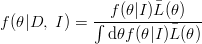


 f(θ|I)¯L(θ) f(θ|D, I) = ∫---------¯---- d θf(θ|I)L(θ)
(21.15)

where we have introduced the quasi-likelihood


 ∫∫<br />¯L (θ) = dηdu L (θ, η, u )h (η, u |θ, I)
(21.16)

Inserting 21.12 into 21.16 and expanding, we have


 [ ¯L(θ) = ∫∫ dηdu h (η, u |θ, I) unL(θ) + un- 1(1 - u) ∑n B (x |η)L (θ) n-2 2∑ j=1 j j +u (1 - u) j<k B (xj|η )B (xk|η)Ljk(θ) + ⋅⋅⋅ + (1 - u)nB (x1|η)⋅⋅⋅B (xn|η)]
(21.17)

in which


 ∏n L(θ) ≡ ∏ i=1 G(xi|θ) Lj(θ) ≡ ni⁄=j G(xi|θ) Lj(θ) ≡ ∏n G (xi|θ)... etc.  i⁄=j,k
(21.18)

are a sequence of likelihood functions for the good distribution in which we use all the data, all except the datum xj, all except xj and xk, and so on. To interpret the lengthy expression 21.17, note that the coefficient of L(θ),


∫ 1 ∫ ∫ du dη h(η, u|θ, I)un = du unh(u|θ, I) 0
(21.19)

is the probability, conditional on θ and the prior information, that all the data {x1,…,xn} are good. This is represented in the Laplace-de Finetti form 21.7 in which the generating function g(u) is the prior density h(u|θ, I) for u, conditional on θ. Of course, in most real problems this would be independent of θ (which is presumably some parameter referring to an entirely different context than u); but preserving generality for the time being will help bring out some interesting points later.

Likewise, the coefficient of Lj(θ) in 21.17 is


∫ ∫ du un- 1(1 - u ) dη B(xj|η)h(η, u|θ, I)
(21.20)

now the factor


 ∫ n-1 d η du u (1 - u)h (η, u |θ I)
(21.21)

is the joint probability density, given I and θ, that any specified datum xj is bad, that the (n- 1) others are good, and that η lies in (η,η + dη). Therefore the coefficient 21.20 is the probability, given I and θ, that the jth datum would be bad and would have the value x
j
, and the other data would be good. Continuing in this way, we see that, to put it in words, our quasi-likelihood is:


¯L (θ ) = prob(all the data are good) × (likelihood using all the data) + ∑ prob(only xjbad) × (likelihood using all data except xj) ∑ j + j,k prob(only xj, xkbad ) × (likelihood using all except xj,xk) + ⋅∑⋅⋅ + j prob(only xj good) × (likelihood using only the datum xj) + prob(all the data are bad )
(21.22)

In shorter words: the quasi-likelihood L¯(θ) is a weighted average of the likelihoods for the good distribution G(x|θ) resulting from every possible assumption about which data are good, and which are bad, weighted according to the prior probabilities of those assumptions. We see how every detail of our prior knowledge about how the data are being generated is captured in the Bayesian solution.

This result has such wide scope that it would require a large volume to examine all its implications and useful special cases. But let us note how the simplest ones compare to our intuition.


21.6 Pure Outliers

Suppose the good distribution is concentrated in a finite interval


G (x|θ) = 0, |x| > 1
(21.23)

while the bad distribution is positive in a wider interval which includes this. Then any datum x for which |x| > 1 is known with certainty to be an outlier, i.e. to be bad. If |x| < 1, we cannot tell with certainty whether it is good or bad. In this situation our intuition tells us quite forcefully: Any datum that is known to be bad is just not part of the data relevant to estimation of θ and we shouldn’t be considering it at all. So just throw it out and base our estimate on the remaining data.

According to Bayes’ theorem this is almost right. Suppose we find xj = 1.432, xk = 2.176, and all the other x’s less than unity. Then, scanning 21.24 it is seen that only one term will survive:


 ∫ ∫ ¯ L(θ) = du dηh (η, u|θ, I)B (xj|η)B (xk |η)Ljk (θ ) = Cjk (θ)Ljk(θ)
(21.24)

As discussed above, the factor Cjk is almost always independant of θ, and since constant factors are irrelevant in a likelihood, our quasi-likelihood in 21.15 reduces to just the one obtained by throwing away the outliers, in agreement with that intuition.

But it is conceivable that in rare cases Cjk(θ) might, after all, depend on θ; and Bayes’ theorem tells us that such a circumstance would make a difference. Pondering this, we see that the result was to be expected if only we had thought more deeply. For if the probability of obtaining two outliers with values xj, xk depends on θ, then the fact that we got those particular outliers is in itself evidence relevant to inference about
θ.

Thus, even in this trivial case Bayes’ theorem tells us something that unaided intuition did not see: even when some data are known to be outliers, their values might still, in principle, be relevant to estimation of θ. This is an example of what we meant in saying that Bayes’ theorem relentlessly seeks out and exposes every factor that has any relevance at all to the question being asked.

In the more usual situations, Bayes’ theorem tells us that whenever any datum is known to be an outlier, then we should simply throw it out, if the probability of getting that particular outlier is independent of θ. For, quite generally, a datum xi can be known with certainty to be an outlier ony if G(xi|θ) = 0 for all θ; but in that case every likelihood in 21.24 that contains xi will be zero, and our posterior distribution for θ will be the same as if the datum xi had never been observed.


21.7 One receding datum

Now suppose the parameter of interest is a location parameter, and we have a sample of ten observations. But one datum xj moves away from the cluster of the others, eventually receding out 100 standard deviations of the good distribution G. How will our estimate of θ follow it? The answer depends on which model we specify.

Consider the usual model in which the sampling distribution is taken to be simply G(x|θ) with no mention of any other ’bad’ distribution. If G is Gaussian, x ≈ N(θ,σ), and our prior for θ is wide (say > 1000σ), then the Bayesian estimate for quadratic loss function will remain equal to the samaple average, and our far-out datum will pull the estimate about ten standard deviations away from the average indicated by the other nine data values. This is presumably the reason why Bayesian methods are sometimes charged with failure to be robust/resistant.

However, that is the result only for the assumed model, which in effect proclaims dogmatically: I know in advance that u = 1; all the data will come from G, and I am so certain of this that no evidence from the data could change my mind. If one actually had this much prior knowledge, then that far-out datum would be highly significant; to reject it as an ’outlier’ would be to ignore cogent evidence, perhaps the most cogent piece of evidence that the data provide. Indeed, it is a platitude that important scientific discoveries have resulted from an experiment having that much confidence in his apparatus, so that surprising new data were believed; and not merely rejected as ’accidental’ outliers.

If, nevertheless, our intuition tells us with overwhelming force that the deviant datum should be thrown out, then it must be that we do not really believe that u = 1 strongly enough to adhere to it in the face of the evidence of the surprising datum. A Bayesian may correct this by use of the more realistic model 21.8. Then the proper criticism of the first procedure is not of Bayesian methods, but rather of the saddling of Bayesian methodology with an inflexible, dogmatic model which denies the possibility of outliers. We saw in Section 4.4 on multiple hypothesis testing just how much difference it can make when we permit the robot to become skeptical about an overly simple model.

Bayesian methods have inherent in them all the desirable robust/resistant qualities, and they will exhibit these qualities automatically, whenever they are desirable – if a sufficiently flexible model permits them to do so. But neither Bayesian nor any other methods can give sensible results if we put absurd restrictions on them. There is a moral in this, extending to all of probability theory. In other areas of applied mathematics, failure to notice some feature (like the possibility of the bad distribution B) means only that it will not be taken into account. In probability theory, failure to notice some feature may be tantamount to making irrational assumptions about it.

Then why is it that Bayesian methods have been criticized more than orthodox ones on this issue? For the same reason that city B may appear in the statistics to have a higher crime rate than city A, when the fact is that city B has a lower crime rate, but more efficient means for detecting crime. Errors undetected are errors uncriticized.

Like any other problem in this field, this can be further generalized and extended endlessly, to a three-model model, putting parameters in 21.6, etc. But our model is already general enough to include both the problem of outliers and conventional hypothesis testing theory; and a great deal can be learned from a few of its simple special cases.

Saturday, December 12, 2009

Stealthy UAVs and Drone Wars

USAF Stealth UAV Has Ties To Previous Designs.

Aerospace Daily and Defense Report (12/10, Fulghum) reported the recently-revealed USAF stealth RQ-170 has "linkages to earlier designs from Lockheed Martin's Advanced Development Programs, including the stealthy DarkStar and Polecat UAVs." The RQ-170 has a "tailless flying wing" featuring communication sensors and is currently serving in Afghanistan.

Drones Being Used Successfully In Pakistan.

On its "Danger Room" blog, Wired (12/10, Schactman) reported on the US military's use of drones in the Afghanistan and Pakistan. According to some estimates, drones have killed "as many as a thousand people" around Pakistan. While America is currently not invading Pakistan, the drones are allowed to pursue militants as long as "the government in Islamabad [is] notified first." These drone strikes are "widely credited for taking out senior leaders of both the Pakistani Taliban and Al Qaeda," but have been criticized as an "extension of the war in Central Asia fought under uncertain authority and with questionable morality."


That "questionable morality" comment is just a smear, but it is interesting stuff anyway.

Friday, December 11, 2009

Lord Monckton on Climategate

Pointed at by theAirVent:

Lord Monckton on Climategate at the 2nd International Climate Conference from CFACT EUROPE on Vimeo.


Gore isn't the only one who can make propaganda...just for entertainment purposes, don't go re-jiggering your economy based on this video, but enjoy.

Ha ha, traffic light tendency:


Calling those guys from East Anglia crooks is a bit over the top (they are just stealth advocates), but it's still entertaining.

Do you validate?


To sum up:

Indeed, much of what is presented as hard scientific evidence for the theory of global warming is false. "Second-rate myth" may be a better term, as the philosopher Paul Feyerabend called science in his 1975 polemic, Against Method.

"This myth is a complex explanatory system that contains numerous auxiliary hypotheses designed to cover special cases, as it easily achieves a high degree of confirmation on the basis of observation," Feyerabend writes. "It has been taught for a long time; its content is enforced by fear, prejudice and ignorance, as well as by a jealous and cruel priesthood. Its ideas penetrate the most common idiom, infect all modes of thinking and many decisions which mean a great deal in human life ... ".
Times Higher Education -- Beyond Debate?

Dueling Bayesians

Percontations: The Nature of Probability

Interest points:

  • Fun with coin-flipping (13:43)

  • Can probabilistic thinking be completely automated? (04:31)

  • The limits of probability theory (11:07)

  • How Andrew got shot down by Daily Kos (06:55)

  • Is the academic world addicted to easy answers? (11:11)

    This part of the discussion was very brief, but probably the most interesting. What Gelman is referring to is maximum entropy sampling, or optimal sequential design of experiments. This has some cool implications for model validation I think (see below).

  • The difference between Eliezer and Nassim Taleb (06:20)


Links mentioned:


Some things Dr Gelman said that I think are interesting:

I was in some ways thinking like a classical statistician, which was, well,I'll be wrong 5% of the time, you know, that's life. We can be wrong a lot, but you're never supposed to knowingly be wrong in Bayesian statistics. If you make a mistake, you shouldn't know that you made a mistake, that's a complete no-no.


With great power comes great responsibility. [...] A Bayesian inference can create predictions of everything, and as a result you can be much more wrong as a Bayesian than as a classical statistician.


When you have 30 cases your analysis is usually more about ruling things out than proving things.

Towards the end of the discussion Yudowski really sounds like he's parroting Jaynes (maybe they are just right in the same way).

Bayesian design of validation experiments

As I mentioned in the comments about the Gelman/Yudowski discussion, the most interesting thing to me was the ’adaptive testing’ that Gelman mentioned. This is a form of sequential design of experiments , and the Bayesian versions are the most flexible. That is because Bayes theorem provides a consistent and coherent (if not always conveneint) way of updating our knowledge state as each new test result arrives. Then, and Gelman’s comment about ’making predictions about everything’ is germane here, we assess our predictive distributions and find the areas of our parameter space that have the most uncertainty (highest entropy of the predictive distribution). This place in our parameter space with the highest predictive distribution entropy is where we should test next to get the most information. The example of academic testing that Gelman gives does exactly that, the question chosen is the one that the test-taker has equal chance of getting right or wrong.

The same idea applies to testing to validate models. Here’s a little passage from a relevant paper that provides some background and motivation [1]:

Under the constraints of time, money, and other resources, validation experiments often need to be optimally designed for a clearly defined purpose, namely computational model assessment. This is inherently a decision theoretic problem where a utility function needs to be first defined so that the data collected from the experiment provides the greatest opportunity for performing conclusive comparisons in model validation.

The method suggested to achieve this is based on choosing a test point from the area of the parameter space with the highest predictive entropy and also one from the area with the lowest predicitive entropy [2]. This addresses the little comment Gelman made about not being able to asses the goodness of the model very well if you only choose points in the high entropy area. Each round of two test points gives you an opportunity to make the most conclusive comparison of the model prediction to reality.

If you were just trying to calibrate a model, then you would only want to choose test points in the high-entropy-areas because these would do the most to reduce your uncertainty about the reality of interest (and hence give you better parameter estimates). Since we are trying to validate the model though, we want to evaluate its performance where we expect it to give the best predictions and where we expect it to give the worst predictions. Here the idea explained in a bit more technical language [1]:

Consider the likelihood ratio Λ(y) in Eq. (9) [or Bayes factor in [6]] as a validation metric. Suppose an experiment is conducted with the minimization result, and the experimental output is compared with model prediction. We expect a high value Λ(y)min , where the subscript min indicates that the likelihood is obtained from the experimental output in the minimization case. If Λ(y)min < η, then clearly this experiment rejects the model, since the validation metric Λ(y), even under the most favorable conditions, does not meet the threshold value η. On the other hand, suppose an experiment is conducted with the maximization result, and the experimental output is compared with the model prediction. We expect a low value Λ(y)max < η in this case. If Λ(y)max > η, then clearly this experiment accepts the model, since it is performed under the worst condition and still produces the validation metric to be higher than η. Thus, the cross entropy method provides conclusive comparison as opposed to an experiment at any arbitrary point.


Here's a graphical depiction of the placement of the optimal Bayesian decision boundary (image taken from [3]):


It would be nice to see these sorts of decision theory concepts applied to the public policy decisions that are being driven by the output of computational physics codes.

References

[1] Jiang, X., Mahadevan, S., “Bayesian risk-based decision method for model validation under uncertainty,” Reliability Engineering & System Safety, No. 92, pp 707-718, 2007.

[2] Jiang, X., Mahadevan, S., “Bayesian cross entropy methodology for optimal design of validation experiments,” Measurement Science & Technology, 2006.

[3] Jiang, X., Mahadevan, S., “Bayesian validation assessment of multivariate computational models ,” Journal of Applied Statistics, Vol. 35, No. 1, Jan 2008.

Thursday, December 10, 2009

Successful Vortex Hybrid Test

Orbital Technologies announced on 8 Dec 2009 that it successfully static tested its big vortex hybrid rocket motor. What's a 'vortex hybrid'? It's a hybrid that controls the fuel regression rate and combustion stability by swirling or recirculating the oxygen that is injected into the cavity of the fuel grain.

The effect of swirling or recirculating the oxygen injection is seen in the photos below taken from this paper:


And here's a little CFD marketing snapshot taken from
Orbital's vortex hybrid data sheet:


And finally here's a nice photo of the test from the ORBITEC press release:

Wednesday, December 9, 2009

Verification, Validation, and Uncertainty Quantification

Notes on Chapter 8: Verification, Validation, and Uncertainty Quantification by George Em Karniadakis [1]. Karniadakis provides the motivation for the topic right off:

In time-dependent systems, uncertainty increases with time, hence rendering simulation results based on deterministic models erroneous. In engineering systems, uncertainties are present at the component, subsystem, and complete system levels; therefore, they are coupled and are governed by disparate spatial and temporal scales or correlations.

His definitions are based on those published by DSMO and subsequently adopted by AIAA and others.

Verification is the process of determining that a model implementation accurately represents the developers conceptual description of the model and the solution to the model. Hence, by verification we ensure that the algorithms have been implemented correctly and that the numerical solution approaches the exact solution of the particular mathematical model typically a partial differential equation (PDE). The exact solution is rarely known for real systems, so “fabricated” solutions for simpler systems are typically employed in the verification process. Validation, on the other hand, is the process of determining the degree to which a model is an accurate representation of the real world from the perspective of the intended uses of the model. Hence, validation determines how accurate are the results of a mathematical model when compared to the physical phenomenon simulated, so it involves comparison of simulation results with experimental data. In other words, verification asks “Are the equations solved correctly?” whereas validation asks “Are the right equations solved?” Or as stated in Roache (1998) [2], “verification deals with mathematics; validation deals with physics.”

He addresses the constant problem of validation succinctly:

Validation is not always feasible (e.g., in astronomy or in certain nanotechnology applications), and it is, in general, very costly because it requires data from many carefully conducted experiments.

Getting decision makers to pay for this experimentation or testing is especially problematic when they were initially sold on using modeling and simulation as a way to avoid testing.

After this the chapter goes into an unnecessary digresion on inductive reasoning. An unfortunate common thread that I’ve noticed in many of the V&V reports I’ve read is they seem to think Karl Popper had the last word on scientific induction! I think the V&V community would profit greatly by studying Jayne’s theoretically sound pragmatism. They would quickly recognize that the ’problems’ they perceive in scientific induction are little more than misunderstandings of probability theory as logic.

The chapter gets back on track with the discussion of types of error in simulations:

Uncertainty quantification in simulating physical systems is a much more complex subject; it includes the aforementioned numerical uncertainty, but often its main component is due to physical uncertainty. Numerical uncertainty includes in addition to spatial and temporal discretization errors, errors in solvers (e.g., incomplete iterations, loss of orthogonality), geometric discretization (e.g., linear segments), artificial boundary conditions (e.g., infinite domains), and others. Physical uncertainty includes errors due to imprecise or unknown material properties (e.g., viscosity, permeability, modulus of elasticity, etc.), boundary and initial conditions, random geometric roughness, equations of state, constitutive laws, statistical potentials, and others. Numerical uncertainty is very important and many scientific journals have established standard guidelines for how to document this type of uncertainty, especially in computational engineering (AIAA 1998 [3]).

The examples given for effects of ’uncertainty propagation’ are interesting. The first is a direct numerical simulation (DNS) of turbulent flow over a circular cylinder. In this resolved simulation, the high-wave numbers (smallest scales) are accurately captured, but there is disagreement at the low wave numbers (largest scales). This somewhat counter-intuitive result occurs because the small scales are insensitive to experimental uncertainties about boundary and initial conditions, but the large scales of motion are not.

The section on methods for dealing with modelling uncertain inputs is sparse on details. Passing mention is made of Monte Carlo and Quasi-Monte Carlo methods, sensitivity-based methods and Bayesian methods.

The section on ’Certification / Accreditation’ is interesting. Karniadakis recomends designing experiments for validation based on the specific use or application rather than based on a particular code. This point deserves some emphasis. It is an often voiced desire from decision makers to have a repository of validated codes that they can access to support their various and sundry efforts. This is an unrealistic desire. A code can not be validated as such, only a particular use of a code can be validated. In most decisions that engineering simulation supports, the use is novel (research and new product development), therefore the validated model will be developed concurrently with (in the case of product development) or as a result of (in the case of research) the broader effort in question.

The suggested hierarchical validation framework is similar to the ’test driven development’ methodologies in software engineering and the ’knowledge driven product development’ championed in the GAO’s reports on government acquisition efforts. Small component (unit) tests followed by system integration tests and then full complex system tests. When the details of ’model validation’ are understood, it is clear that rather than replacing testing, simulation truly serves to organize test designs and optimize test efforts.

The conclusions are explicit (emphasis mine):

The NSF SBES report (Oden et al. 2006 [4]) stresses the need for new developments in V&V and UQ in order to increase the reliability and utility of the simulation methods at a profound level in the future. A report on European computational science (ESF 2007 [5]) concludes that “without validation, computational data are not credible, and hence, are useless.” The aforementioned National Research Council report (2008) on integrated computational materials engineering (ICME) states that, “Sensitivity studies, understanding of real world uncertainties and experimental validation are key to gaining acceptance for and value from ICME tools that are less than 100 percent accurate.” A clear recommendation was reached by a recent study on Applied Mathematics by the U.S. Department of Energy (Brown 2008 [6]) to “significantly advance the theory and tools for quantifying the effects of uncertainty and numerical simulation error on predictions using complex models and when fitting complex models to observations.”

References

[1] WTEC Panel Report on International Assessment of Research and Development in Simulation-Based Engineering and Science, 2009, http://www.wtec.org/sbes/SBES-GlobalFinalReport.pdf

[2] Roache, P.J. 1998. Verification and validation in computational science and engineering. Albuquerque,: Hermosa Publishers.

[3] AIAA Guide for the Verification and Validation of Computational Fluid Dynamics Simulations, Reston, VA, AIAA. AIAA-G-077-1998.

[4] Oden, J.T., T. Belytschko, T.J.R. Hughes, C. Johnson, D. Keyes, A. Laub, L. Petzold, D. Srolovitz, and S. Yip. 2006. Revolutionizing engineering science through simulation: A report of the National Science blue ribbon panel on simulation-based engineering science. Arlington: National Science Foundation. Available online

[5] European Computational Science Forum of the European Science Foundation (ESF). 2007. The Forward Look Initiative. European computational science: The Lincei Initiative: From computers to scientific excellence. Information available online.

[6] Brown, D.L. (chair). 2008. Applied mathematics at the U.S. Department of Energy: Past, present and a view to the future. May, 2008.


Concepts of Model Verification and Validation has a glossary that defines most of the relevant terms.
