This previous post covered time-convergence of a single trajectory, and the growth of the spread in an ensemble. The next post covered some special considerations that chaos imposes on us when we try to apply the method of manufactured solutions (MMS). I’ll try to tie up some loose ends in this (perhaps final) installment of the Lorenz63 series. Two questions that I think I haven’t adequately addressed yet:
- What about the time-step convergence behavior of an ensemble?
- So can you successfully apply the MMS to verify implementations of numerical approximations to this system or not? (The literature indicates that you can, but I didn’t actually demonstrate the correctness of my implementation.)
To address the first question I wrote a little Python script that runs a range of trajectories with various time-steps and also perturbations to the initial conditions:
step = [1, 2, 4]
T = 60.0 # integration period
# parameters for the Lorentz 63 system to get chaotic response:
Pr = 10.0
Ra = 28.0
b = 8.0 / 3.0
# knobs for the Newton’s method:
tol = 1e-14
maxits = 20
# number of different IC’s in our ensemble:
nic = 5
# number of pairs of differences between ensemble members:
npairs = comb(nic, 2, exact=1)
h = []
x = []
xdiffs = []
y = []
ydiffs = []
z = []
zdiffs = []
t = []
for n in nt:
h.append(T / float(n))
x.append(sp.zeros((n,nic), dtype=float, order=’F’))
xdiffs.append(sp.zeros((n,npairs), dtype=float, order=’F’))
y.append(sp.zeros((n,nic), dtype=float, order=’F’))
ydiffs.append(sp.zeros((n,npairs), dtype=float, order=’F’))
z.append(sp.zeros((n,nic), dtype=float, order=’F’))
zdiffs.append(sp.zeros((n,npairs), dtype=float, order=’F’))
t.append(sp.linspace(0.0, T, n))
# some perturbations:
eps = 1e-16 * sp.array([0, 1, -1, 2, -2])
for i in xrange(len(nt)):
x[i][0,:] = 1.0 + eps
y[i][0,:] = -1.0 + eps
z[i][0,:] = 10.0 + eps
# calculate all of the trajectories:
for i in xrange(len(nt)): # time-step variation loop
for j in xrange(nic): # perturbations loop
L63.time_loop(
x[i][:,j],y[i][:,j],z[i][:,j],t[i],Ra,Pr,b,h[i],tol,maxits)
Here the result for the x-component of the solution:
Figure 1 shows that we have a time-step converged solution out to t ≈ 30. After which, the trajectory between the different time-steps is significantly different, but the ensemble spread is still negligible. At t ≈ 40 the ensemble begins to spread noticeably for all three time-step sizes, and then shortly thereafter we get an abrupt divergence of the trajectories for all of the ensemble members.
The interesting question is whether the divergence is inevitable (that’s my impression from reading the ’chaos’ literature, let me know if you think/know something different), or if getting more and more accurate solutions will delay that abrupt divergence (the visible divergence seems to happen latter in the most resolved ensemble). Unfortunately, I’m already flirting with swap-thrash on my little laptop with these ensembles, so I need to do a little re-factoring before I’ll be able to demonstrate that one definitively (so this probably isn’t the final installment). What’s really required here is a time-step converged solution of the region t > 40 where the ensemble members diverge. These solutions aren’t there yet (smaller time-step or higher-order method is needed).
The second part of the post will deal with demonstrating an MMS-based verification of my (purportedly third-order accurate) implementation. As discussed in this post, since the system is chaotic, choosing a manufactured solution becomes a bit more difficult. Here’s a Python script which calculates trajectories with MMS forcing and calculates error norms:
step = [1, 2, 4, 8, 16]
T = 2.0 * sp.pi # integration period
Pr = 10.0
Ra = 28.0
b = 8.0 / 3.0
tol = 1e-14
maxits = 20
mms_switch = 1
h = []
x = []
y = []
z = []
t = []
ms = []
for n in nt:
h.append(T / float(n)) # time-step size
x.append(sp.zeros(n, dtype=float, order=’F’))
y.append(sp.zeros(n, dtype=float, order=’F’))
z.append(sp.zeros(n, dtype=float, order=’F’))
t.append(sp.linspace(0.0, T, n))
ms.append(sp.zeros((n,3), dtype=float, order=’F’))
bx = 0.0
by = -1.0
bz = 10.0
# manufactured solutions:
for i in xrange(len(nt)):
ms[i][:,0] = sp.cos(t[i]) + bx
ms[i][:,1] = sp.sin(t[i]) + by
ms[i][:,2] = sp.sin(t[i]) + bz
# trajectories:
for i in xrange(len(nt)):
x[i][0] = bx + 1.0
y[i][0] = by
z[i][0] = bz
L63.time_loop(
x[i],y[i],z[i],t[i],Ra,Pr,b,h[i],tol,maxits,mms_switch,bx,by,bz)
# error L2 norms:
err_x = sp.zeros(len(nt), dtype=float)
err_y = sp.zeros(len(nt), dtype=float)
err_z = sp.zeros(len(nt), dtype=float)
for i in xrange(len(nt)):
err_x[i] = sp.sqrt(sp.sum((x[i] - ms[i][:,0])**2)/nt[i])
err_y[i] = sp.sqrt(sp.sum((y[i] - ms[i][:,1])**2)/nt[i])
err_z[i] = sp.sqrt(sp.sum((z[i] - ms[i][:,2])**2)/nt[i])
# find the observed order of convergence:
px = sp.polyfit(sp.log(h), sp.log(err_x), 1)
py = sp.polyfit(sp.log(h), sp.log(err_y), 1)
pz = sp.polyfit(sp.log(h), sp.log(err_z), 1)
Figure 2 shows the behavior of the solution with MMS forcing when the manufactured solution is not in the convergent region. The solution really is not converging.
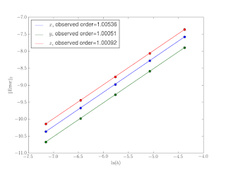
Contrast this with the behavior in Figure 3, which actually shows at least first order convergence (and the solution looks like the one we chose).
The fact that the slope of the line in Figure 3 is 1 rather than 3 means I still have a lurking ordered-error in my implementation (likely in the error calculations themselves), or I’m not yet in the asymptotic range, though this seems unlikely given the small time-step size and very consistent slope. The good news illustrated by Figure 3 is that we can apply MMS to even chaotic systems. Now where’s that bug…


No comments:
Post a Comment