Saturday, January 24, 2009

Convective Flux Jacobians

The Euler equations are an important system of equations in computational fluid dynamics (CFD). They are basically the full continuum equations of motion without the viscosity. Adding in the viscosity gives you the more realistic Navier-Stokes equations.

The conserved variable vector is

And the flux vector is

The flux Jacobian is simply the partial derivative of the flux with respect to the conserved variables (mass, momentum, energy).

The maxima to calculate the Jacobian is straightforward:

U : matrix([u1], [u2], [u3]);

f1 : u2;
f2 : u2^2 / u1 + p_exp;
f3 : (u2 / u1) * (u3 + p_exp);
F : matrix([f1], [f2], [f3]);

A : zeromatrix(nd, nd);

for j : 1 thru nd do
(
for i : 1 thru nd do
(
A[i,j] : diff(F[i,1], U[j,1])
)
);


Diagonalization


Using the chain rule lets you write the Euler equations in a quasi-linear form in terms of the flux Jacobian, now called A.

The flux Jacobian can be diagonalized into a matrix of right eigenvectors, diagonal matrix of eigenvalues, and a matrix of left eigenvectors.

The code to accomplish this in maxima is a little more involved, because of some substitutions needed to get everything in terms of u,gamma,a.

load("eigen");
VLV : eigenvectors(simp_A);

a_exp : (g * (g - 1) / u1) * (u3 - u2^2 / (2 * u1));
a_exp : sqrt(a_exp);
simp_a : ratsimp(ev(a_exp, u1 = rho, u2 = rho * u, u3 = rho * E));
a_eqn : a^2 = simp_a^2;
c_exp : g*(2*E-u^2);
a_eqn : facsum(a_eqn, c_exp);

/* put the eigenvectors into a matrix: */
V : columnvector( VLV[2] );
V : addcol( V,VLV[3],VLV[4] );
V : ratsimp( V );

/* put the eigenvalues into a diagonal matrix: */
load("diag");
L : diag( VLV[1][1] );

radsubstflag : true;
/* substitute in the speed of sound: */
V : ratsimp(ratsubst(a, simp_a, ratsimp(V)));
V : factor(ratsimp(ratsubst(a, simp_a, rootscontract(V))));
/* factor out gammas */
V : facsum(V,g);
c_a : part(solve(ratsubst(c,c_exp,a_eqn),c)[1],2);
V : ratsubst(c,c_exp,V);
V : ratsubst(ev(c_a),c,V);
V : facsum(V,u);

/* substitute in the speed of sound: */
L : ratsimp(ratsubst(a, simp_a, ratsimp(L)));

/* left eigenvectors: */
Vinv : factor( ratsimp( invert( V ) ) );
/* factor out gammas */
Vinv : facsum(Vinv,g);
d_exp : (g-1)/a^2;
Vinv : ratsubst(d,d_exp,Vinv);

Conclusion


The thing to note about this result is that there are three distinct wave speeds in the one dimensional Euler equations, u-a, u+a, and u, where a is the speed of sound. There are lots of possible ways to write the eigenvectors, in terms of the enthalpy, or the energy, or the pressure, but the form above with only the flow velocity, the speed of sound, and the ratio of specific heats is pretty elegant. It really illustrates what a fundamental quantity the speed of sound is for this set of equations.

Chapter 3 of Riemann Solvers and Numerical Methods for Fluid Dynamics: A Practical Introduction has a good work-up of this development and shows some alternative formulations for the flux Jacobian.
Sunday, January 11, 2009

Kronecker Product of Sparse Matrices

Gilbert Strang discusses the use of a neat built-in function in Octave, kron(), that's pretty useful for doing multidimensional finite difference methods on PDEs:


kron() takes the Kroenecker product of two matrices. This is especially useful when constructing the large, sparse matrices needed for finite difference approximations.

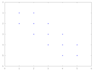
K is the tridiagonal matrix created for a central difference approximation to the second derivative:

n = 5;
K = spdiag(2*ones(n,1),0) + spdiag(-ones(n-1,1),-1) + spdiag(-ones(n-1,1),1);
spy(K)


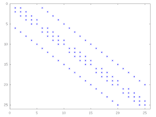
K is the differences for a 1D row of points, now we can create the 2-dimensional version for a plane of points with kron():

K2D = kron(speye(n),K) + kron(K,speye(n));
spy(K2D);


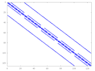
The extension to 3 dimensions is exactly as before, now we have a matrix describing the differences between points on the same line in the first sub and superdiagonal, differences across lines in the next bands out from those, and differences across planes in the furthest out bands:

K3D = kron(speye(n),K2D) + kron(K2D,speye(n));
spy(K3D);

Pretty simple! Now you're ready to solve multidimensional partial differential equations.

Friday, January 9, 2009

Fibonacci Numbers

Gilbert Strang has an interesting example in one of his linear algebra lectures on eigenvalues that is relevant to the articles I've written on speeding up calculations in Octave.

You might be familiar with the Fibonacci numbers, they are calculated by a two term recurrence:


We've already seen that recasting a calculation in terms of a matrix vector multiply or matrix vector solve is an important skill for writing good fast code in Octave. Strang demonstrates this at about halfway through the above lecture. The first order system that describes the generation of Fibonacci numbers is:


The nth term of the sequence is calculated by taking the nth power of A and applying it to the initial conditions:


When you diagonalize a matrix the powers of the matrix become very easy to calculate:

If you aren't familiar with the concept of eigenvalues and eigenvectors and diagonalizing a matrix I would highly recommend the linear algebra lectures on MIT's OCW website.

Here's the Octave code to accomplish the above. If you want, you can use tic() and toc() for timing. On my laptop the matrix method is about three times faster than the for loop method. What kind of results do you get? This advantage will grow as you go further into the sequence because the amount of work stays constant for the matrix method, but grows linearly for the recurrence method.

%% Our 'fibonacci' operator:
A = [1,1;1,0]
%% our initial conditions:
u_0 = [0;1];

%% get the matrix of eignevectors, V, and the matrix of eigenvalues, lambda
[V,lambda] = eig(A)

%% A = V lambda V^{-1}

Vinv = inverse(V)

%% This gives us an idea of the error introduced by calculating the
%% inverse with finite precision arithmetic:
Error = A - V*lambda*Vinv

n = 1400;
F = zeros(n,2);
%% Find the 100th Fibonaci number:
F(100,:) = V * (lambda^100) * Vinv * u_0;

%% check our answer with a simple loop:
fibo = zeros(n,1);
fibo(1) = 0;
fibo(2) = 1;
for i=3:n
fibo(i) = fibo(i-1) + fibo(i-2);
endfor

for i=2:n
F(i,:) = V * (lambda^i) * Vinv *u_0;
endfor

relative_error = abs( ( F(3:n,2) - fibo(3:n) ) ./ fibo(3:n) );

One thing to note is that one of the eigenvalues of our matrix is greater than one. This has implications for the numerical stability of the above method for calculating terms in the Fibonacci sequence. It means that the initial tiny round-off error in our eigenvector matrix inverse will be amplified as we continue to calculate higher and higher terms in the sequence. This behaviour is shown in the plot below, luckily the error starts out very small, and doesn't grow too large before we run out of range in the 32bit floating point numbers on the machine.

What's the answer? The 100th Fibonacci number is approximately 2.1892e20.

Monday, January 5, 2009

How to Speed Up Octave

Speed seems like a continuing theme on the Octave mailing lists, a recent thread on the list of "comparing the executive speed with Matlab" demonstrates that there really is very little speed overhead when you use Octave smartly. If you read down far enough, it also demonstrates that the Intel Fortran compiler is awesome!

There are four basic methods of speeding up a chunk of Octave code (in order of increasing speed):
  1. Allocate memory smartly (using for loops)

  2. Vectorize your code (avoiding for loops)

  3. Use sparse matrix operators in place of for loops you can't vectorize

  4. Write a compiled function in C/C++/Fortran to call from Octave

The first three options keep you in pure Octave. The fourth option, while requiring you to use a compiled language is really not too bad because you can use all of the types (vectors, matrices, etc) defined in the Octave libraries to write your function. That's almost as easy as doing it in Octave.

Speeding Up For Loops


This one really amounts to not being foolish. The only way to speed up for loops is to make sure you allocate all of your memory (using zeros() for instance) before you enter the for loop. The Octave Manual covers this topic here. The better thing to do is vectorize your code and avoid for loops all together.

Vectorizing


What you really want to do is cast your calculation as a series of vector and matrix operations, or use the built-in (usually compiled) functions that operate directly on vectors. The post Is Octave Slow? demonstrates the sorts of speed up you can get when you get rid of for loops.

Sparse Matrices for Data Dependancy


What about for loops you can't vectorize? The ones where the result at iteration n depends on what you calculated in iteration n-1, n-2, etc. You can define a sparse matrix that represents your for loop and then do a sparse matrix solve. This is much faster because you are now using compiled functions. The drawback is that you are trading some increase (sometimes substantial) in memory usage to buy this speed up.


Compile It


The manual has a good intro on using mkoctfile to compile your function and make it callable from Octave. Probably the most useful thing is that you can use the Octave types, so you don't have to code up your own matrix or vector type. At this point the speed really has little to do with Octave and everything to do with the quality of the compiler you use and how efficiently you code up your calculation.

Conclusion


The real power of Octave isn't that you can get your calculations to be nearly as fast as if you wrote them all in a compiled language. It's that you can prototype a calculation quickly and make sure that it is correct, and then there is a fairly well defined path to follow to speed up your correct calculation.

Saturday, January 3, 2009

Thresholding for Edge Detection

The real world is noisy, and the differencing operations of edge detection tend to magnify that noise. We can apply some statistical methods to our edge detection to hopefully overcome that. A very basic approach is to threshold based on a histogram of the gradient magnitude. Taking a look at the distribution of gradient magnitude for our trusty old electricity meter (shown below), it looks like a pixel level below about 235 puts us safely out into the tail of the distribution. Most pixels (in this image) are not edge pixels, so they are clustered on the high end of the scale.

This is pretty easy to do with numpy and Image (PIL):

import numpy
import Image
pix = numpy.array( img.getdata() )
for i in xrange(0,pix.size):
if pix[i] < 235: pix[i] = 0 else: pix[i] = 255 img_out.putdata( pix )


Of course the histogram shape will depend on how much noise and how many edges are in the particular picture. This one had black dials on a white background, and not much noise so thresholding is a pretty fruitful strategy for really pulling out the edges.

You can make an intuitive argument that gradient magnitude distributions will have roughly similar shapes to that shown above. Especially as image resolutions steadily increase, the vast majority of pixels will not be on an edge. Sort of the curse of dimensionality in reverse, I guess that makes it a blessing.

Friday, January 2, 2009

Incompatibility between Matplotlib and Numpy

If you are running Fedora 9 you may have run in to this problem (at least one other guy did). Taking a look at the bugzilla over at RedHat shows that this has been a recurring problem over the past couple years (first cropping up in FC5). It seems that the packagers for numpy and matplotlib are having trouble synchronizing the updates for numpy and matplotlib. They are fast moving projects so one occasionally changes the API quietly and breaks the other. Of course there are other dependencies that probably play in to the decision of when to update a particular package, but this is the one that breaks my workflow.

The easiest fix for me was to download the latest matplotlib sources and compile/install them manually:

$ tar -zxvf matplotlib-0.98.5.2.tar.gz
$ cd matplotlib-0.98.5.2
$ python setup.py build
$ su
$ python setup.py install

This is less than ideal, because now I'm not running a "stock" Fedora where all of my software updates are taken care of automagically, but the increase in work-load is negligible.

A work-around for the incompatibility between numpy and matplotlib that requires editing some of the python sources:
http://www.mail-archive.com/numpy-discussion@scipy.org/msg13753.html

Or you can just upgrade to Fedora 10. Unfortunately that's not an option for me because of a closed proprietary device driver that relies on < 2.6.27 kernels. I haven't compiled my own kernels since FC1 days, and don't really feel like getting back into the habit.

Thursday, January 1, 2009

A Treatise on the Calculus of Finite Differences


Boole, George. "A Treatise on the Calculus of Finite Differences", Macmillan and Co., 1872.

The public domain and Google books is a great combination. You can download the classic by George Boole, A Treatise on the Calculus of Finite Differences (TCFD) and read it at your leisure, for free!

Even though it was written in 1860, this book probably even more relevant today than it was then. Why? Because it provides the mathematical basis for solving higher and higher resolution partial differential equations with faster and faster computers for the complex domains of modern engineering problems. The faster, more accurate and more efficient solution to these types of problems provides the foundation for improving quality of life for everyone.

I like his definition of the calculus of finite differences, it says so much, succinctly:
The Calculus of Finite Differences may be strictly defined as the science which is occupied about the ratios of the simultaneous increments of quantities mutually dependant.

This book has to be understood as a second volume to accompany Boole's first book on Differential Equations. He stresses the importance of the relationship between the two in his preface to TCFD. The discussion of the distinction between a calculus of limits and the calculus of differences highlights this connection.

Like most old math or science books, it is the discussion of important applications that feels dated. The ideas are timeless, but the important applications change with the problems and the technology of the time.

Another timeless idea that bears repeating around all practitioners of the numerical art (from Chapter 8):

... we shall very often need to use the method of Finite Differences for the purpose of shortening numerical calculation, and here the mere knowledge that the series obtained are convergent will not suffice; we must also know the degree of approximation.

To render our results trustworthy and useful we must find the limits of the error produced by taking a given number of terms of the expansion instead of calculating the exact value of the function that gave rise thereto.